4.3. Forward And Inversion Workflow Agents#

These agents prepare, run, evaluate, or compare physics-based modelling and inversion workflows. They split cleanly into three roles: ForwardModelAgent applies the forward operator in the direction model → data; InversionPrepAgent, Occam2DAgent, ModEmAgent, and Mare2DEMAgent write native input files for the inverse direction without necessarily running a solver; and InversionBackendAgent, InversionEvaluationAgent, and InversionComparisonAgent run, evaluate, or compare the recovered model. Every runnable example below uses the same 28-station WILLY L18PLT profile as the rest of this guide (data/AMT/WILLY_DATA/L18PLT), loaded once with MTLoaderAgent.

4.3.1. ForwardModelAgent#

ForwardModelAgent applies the forward operator from pycsamt.forward – 1-D, 2-D (finite-difference TE+TM), or quasi-3-D, selected by dim – to a resistivity model. Use it for synthetic checks, sensitivity experiments, or validating how a proposed model should appear in impedance or apparent-resistivity space before it is ever compared against field data. The input dictionary takes freqs (Hz), not periods – passing periods is silently ignored and the agent falls back to its default 40-point log-spaced band, so double-check the key name if a run uses fewer frequencies than requested.

>>> import numpy as np
>>> from pycsamt.agents import ForwardModelAgent

>>> result = ForwardModelAgent(dim=1).execute({
...     "model": {
...         "resistivities": [100.0, 10.0, 1000.0, 100.0],
...         "thicknesses": [500.0, 1000.0, 2000.0],
...     },
...     "freqs": list(np.logspace(-2, 2, 12)),
...     "output_dir": "outputs/forward",
... })
>>> print(result.summary)
1-D forward: 4 layers. no observed data. 1 figure(s).
>>> result["rho_a"][:3]
array([75.39399946, 65.4962356 , 53.51079821])

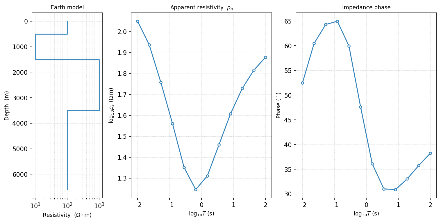
Synthetic 1-D forward model, apparent resistivity, and phase for a four-layer earth. — The three panels `plot_response_and_model_1d` combines: the layered earth model, its synthetic \(\rho_a\), and its synthetic phase – the same round trip used as a sanity check throughout Overview.#

Pass observed sites alongside a 1-D model and the agent also scores the mismatch, using a simpler statistic than the glossary’s general RMS misfit: an unweighted log-apparent-resistivity RMS,

\[\mathrm{RMS}_{\log\rho_a} = \sqrt{\frac{1}{N}\sum_{i=1}^{N} \bigl(\log_{10}\rho_{a,i}^{\mathrm{obs}} - \log_{10}\rho_{a,i}^{\mathrm{fwd}}\bigr)^2},\]

interpolated onto the observed period grid and computed with no per-datum error weighting – useful as a coarse “does this model look plausible at all” check, but not interchangeable with the normalised, uncertainty-aware RMS misfit an actual inversion reports. Comparing the arbitrary four-layer model above against the real WILLY profile (unrelated survey, so a large value is expected) gives exactly that kind of number:

>>> from pycsamt.agents import MTLoaderAgent

>>> loaded = MTLoaderAgent().execute({"path": "data/AMT/WILLY_DATA/L18PLT"})
>>> checked = ForwardModelAgent(dim=1).execute({
...     "model": {
...         "resistivities": [100.0, 10.0, 1000.0, 100.0],
...         "thicknesses": [500.0, 1000.0, 2000.0],
...     },
...     "freqs": list(np.logspace(-2, 2, 12)),
...     "sites": loaded["sites"],
... })
>>> print(checked.summary)
1-D forward: 4 layers. RMS 1.151. 1 figure(s).

An RMS of 1.15 here says only that this arbitrary model is roughly the right order of magnitude for the WILLY profile, not that it is a fitted result – treat it exactly as Overview treats a noiseless round-trip check: confirmation the forward path runs correctly, not evidence about the earth.

4.3.2. InversionPrepAgent#

InversionPrepAgent is meant as the general, backend-agnostic pre-inversion interface – its own module docstring calls it a “Phase 2 stub.” It always validates the Sites object and counts stations and periods; whether it actually writes a file depends entirely on code. Run against the real WILLY profile to see the current state honestly:

>>> from pycsamt.agents import MTLoaderAgent, InversionPrepAgent

>>> loaded = MTLoaderAgent().execute({"path": "data/AMT/WILLY_DATA/L18PLT"})
>>> prep = InversionPrepAgent().execute({
...     "sites": loaded["sites"],
...     "output_dir": "outputs/inversion_prep",
...     "period_range": [0.001, 1.0],
... })
>>> print(prep.status)
needs_review
>>> print(prep.summary)
Inversion prep (occam2d): 28 stations, ~39 periods. No data file written.
>>> print(prep.warnings)
['pycsamt.models.occam2d not available. Data file was not written.']

code="occam2d" (the default) currently cannot write a file at all: the writer function it calls, write_occam2d_data, does not exist in the installed pycsamt.models.occam2d, so every call falls through to the ImportError branch above regardless of input. code="modem" is explicitly stubbed the same way, with its own warning that the ModEM writer is planned for a future phase. n_stations and n_periods in the result are still real and useful for a quick survey-scope check, but for actually writing inversion-ready files today, use Occam2DAgent, ModEmAgent, or Mare2DEMAgent directly – each verified working below.

4.3.3. Occam2DAgent#

Occam2DAgent is the specialized Occam2D preparation agent. It writes the data, mesh, model, and startup files described in Occam2D – the same four-file set, regardless of whether the request goes through this agent or the lower-level writers directly.

Use it after QC, correction, optional rotation, and frequency selection:

>>> from pycsamt.agents import MTLoaderAgent, Occam2DAgent

>>> loaded = MTLoaderAgent().execute({"path": "data/AMT/WILLY_DATA/L18PLT"})
>>> occam = Occam2DAgent().execute({
...     "sites": loaded["sites"],
...     "output_dir": "outputs/willy_occam2d",
...     "run_external": False,
... })
>>> print(occam.summary)
Occam2D prep: 28 stations × 53 periods. 4/4 files written to outputs/willy_occam2d.
>>> sorted(occam.data)
['data_path', 'mesh_path', 'model_path', 'n_data', 'n_periods', 'n_stations', 'output_dir', 'startup_path']

run_external=False stops after writing the four files, so no Occam2D binary is required to reach this success status; set it to True only once that binary is installed and the run should actually execute. This is the same agent, run the same way, already documented in Agent Catalogue; it is repeated here because forward and inversion preparation belong to one physics-based chain, and every reader of that chain should see the exact same numbers in both places.

4.3.4. ModEmAgent#

ModEmAgent prepares ModEM 3-D impedance data files. Use it when the survey and interpretation target require 3-D inversion products rather than a 2-D profile. Unlike InversionPrepAgent’s code="modem" path above, this specialized agent is fully implemented:

>>> from pycsamt.agents import MTLoaderAgent, ModEmAgent

>>> loaded = MTLoaderAgent().execute({"path": "data/AMT/WILLY_DATA/L18PLT"})
>>> modem = ModEmAgent().execute({
...     "sites": loaded["sites"],
...     "output_dir": "outputs/willy_modem",
... })
>>> print(modem.summary)
ModEM3D prep: 28 stations × 53 periods. 4 file(s) written to outputs/willy_modem.
>>> modem["data_path"].name
'ModEM_Data.dat'
>>> modem["model_path"].name, modem["cov_path"].name, modem["ctrl_path"].name
('m0.ws', 'ModEM.cov', 'ModEM.inv')

The four files – data, starting model, covariance, and control – are exactly the ones ModEM documents; model_path, cov_path, and ctrl_path come from a separate InputBuilder step run automatically after the data file, and only ever come back None if that step warns rather than errors (check modem.warnings in that case, since status still reads "success" off the data file alone).

4.3.5. Mare2DEMAgent#

Mare2DEMAgent orchestrates MARE2DEM 2.5-D EM inversion preparation and, when a compiled binary is available, execution. It is the specialized agent to use when the target workflow needs MARE2DEM .emdata, .resistivity, .settings, and run-directory products rather than Occam2D or ModEM files.

The agent can work in three modes:

"prepare": Write input files only. This is the safest default and is appropriate when the run will be launched manually on a workstation or cluster.
"run": Write inputs and launch the configured MARE2DEM binary. Use this only after confirming the binary, MPI configuration, and source tree.
"report": Inspect an existing run directory and summarize result state without writing new inputs or launching the binary.

Typical input keys include emdata for an existing data file, mt or csem dictionaries for building survey data, optional topo, optional resistivity, output_dir, source_dir, n_procs, max_iterations, target_rms, and initial_rho. Build from survey parameters when there is no .emdata file yet, by passing the MARE2DEM survey configuration through mt or csem:

>>> import numpy as np
>>> from pycsamt.agents import Mare2DEMAgent

>>> agent = Mare2DEMAgent(n_procs=8)
>>> prepared = agent.execute({
...     "mt": {
...         "frequencies": list(np.logspace(-3, 3, 20)),
...         "rx_y": list(np.linspace(-5000, 5000, 20)),
...         "rx_type": "land",
...         "lTE": True,
...         "lTM": True,
...     },
...     "topo": 0.0,
...     "output_dir": "outputs/mare2dem",
...     "mode": "prepare",
... })
>>> print(prepared.summary)
MARE2DEM prepare:. 20 MT receivers. 1600 data points. 3/3 files written. Output: outputs/mare2dem.
>>> prepared["data_path"].name, prepared["settings_path"].name
('mare2dem.emdata', 'mare2dem.settings')
>>> prepared["binary_found"]
False
>>> prepared.warnings
['MARE2DEM binary not found. Set download_source=True to auto-build, or run: SourceManager().download(); SourceManager().build()']

binary_found is False and a warning explains why, but status is still "success" – mode="prepare" only needs to write the files, which it did (3/3); reaching that same result with mode="run" instead would require the compiled MARE2DEM binary this environment does not have. Once a .emdata file exists, the second and later runs can reuse it directly instead of rebuilding the survey configuration:

>>> reused = agent.execute({
...     "emdata": "outputs/mare2dem/mare2dem.emdata",
...     "output_dir": "outputs/mare2dem_rerun",
...     "initial_rho": 100.0,
...     "target_rms": 1.0,
... })
>>> print(reused.summary)
MARE2DEM prepare:. 20 MT receivers. 1600 data points. 3/3 files written. Output: outputs/mare2dem_rerun.

Use Mare2DEMAgent after QC, static-shift correction, tensor rotation, and frequency selection. Use InversionEvaluationAgent afterwards when a run directory contains results that need RMS, convergence, or residual summaries.

4.3.6. InversionBackendAgent#

InversionBackendAgent connects agent workflows to the backend-neutral pycsamt.inversion API documented in Overview – builtin, simpeg, pygimli, occam2d, or modem – so a workflow can select or execute a configured backend rather than only write preparation files:

backend = InversionBackendAgent().execute({
    "sites": processed_sites,
    "backend": "occam2d",
    "output_dir": "/out/backend_run",
})

Passing a real, field-derived Sites object is the agent’s documented contract, but as of this writing that specific path does not complete for ordinary field data with the builtin backend, on either dimension:

>>> from pycsamt.agents import MTLoaderAgent, InversionBackendAgent

>>> loaded = MTLoaderAgent().execute({"path": "data/AMT/WILLY_DATA/L18PLT"})
>>> backend = InversionBackendAgent().execute({
...     "sites": loaded["sites"],
...     "backend": "builtin",
...     "dimension": "1d",
... })
>>> print(backend.status)
failed
>>> print(backend.error)
Inversion failed: frequencies must match data sample length.

The failure comes from the internal Sites → EMData adapter, not from the solver itself: real field EDIs rarely share one common frequency grid across every station, and that adapter currently expects one. It is worth knowing precisely because the symptom – a shape-mismatch ValueError – gives no hint that the fix lives upstream of anything this agent’s own parameters (n_layers, max_iter, regularization) can control. Until that adapter is fixed, prefer one of two working paths: write native input files with Occam2DAgent, ModEmAgent, or Mare2DEMAgent (all verified above) and run the external solver directly; or call pycsamt.inversion yourself with an explicit freqs/rho_a/phase dictionary the way Overview does, bypassing the Sites adapter entirely. backend="occam2d" or "modem" inside this same agent additionally require the corresponding external binary to be installed, independent of this data-shape issue.

4.3.7. InversionEvaluationAgent#

InversionEvaluationAgent compares two Sites-shaped collections – observed data against a model-predicted response – to summarize per-station RMS, a residual phase tensor table, and a station-response figure. Its input keys are sites_obs/path_obs and sites_mod/path_mod, both accepting the same kinds of input as MTLoaderAgent; it does not accept an inversion run directory path directly, so a completed Occam2D or ModEM response first needs loading into a Sites-like object. Its RMS statistic is the same unweighted log-apparent-resistivity formula ForwardModelAgent uses above, applied per-station instead of averaged over one model.

There is no fitted model response available in this environment to compare against (see the InversionBackendAgent limitation just above), so the run below compares the WILLY profile with itself – a sanity check on the mechanics, not a real evaluation, exactly as noted for ForwardModelAgent’s self-comparison earlier:

>>> from pycsamt.agents import MTLoaderAgent, InversionEvaluationAgent

>>> loaded = MTLoaderAgent().execute({"path": "data/AMT/WILLY_DATA/L18PLT"})
>>> evaluation = InversionEvaluationAgent().execute({
...     "sites_obs": loaded["sites"],
...     "sites_mod": loaded["sites"],
...     "output_dir": "outputs/willy_eval",
... })
>>> print(evaluation.summary)
Inversion evaluation: global RMS = 0.000
>>> list(evaluation["rms_per_station"].items())[:3]
[('18-001A', 0.0), ('18-002U', 0.0), ('18-003A', 0.0)]

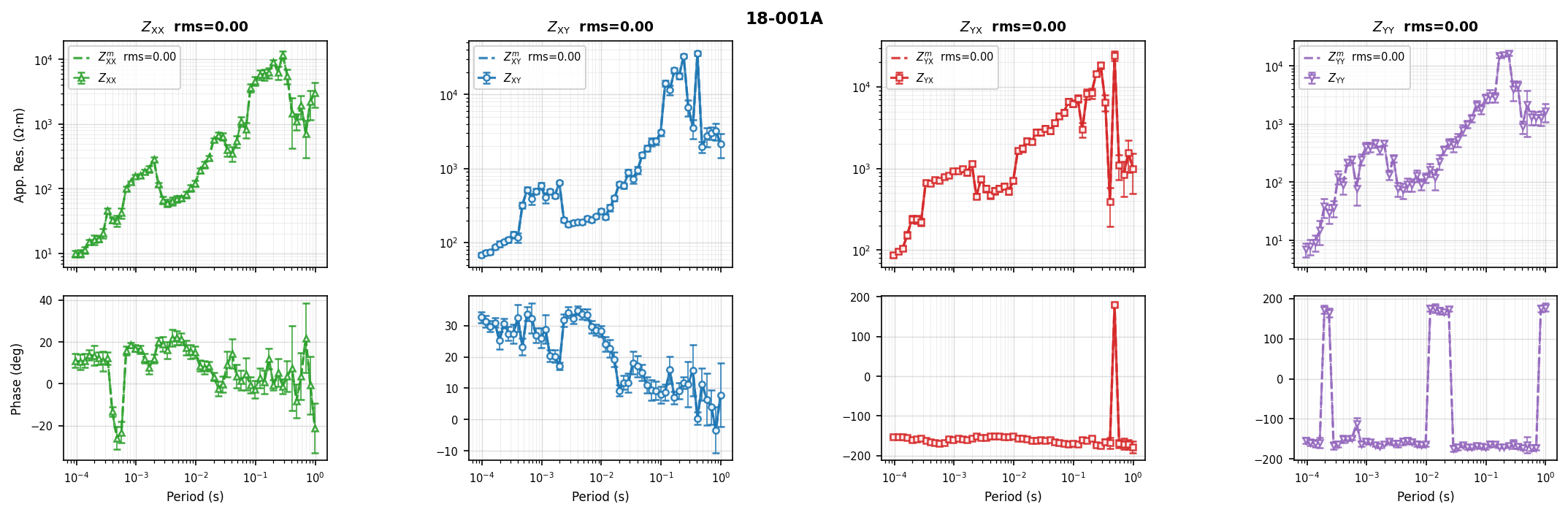
Observed versus model apparent resistivity and phase for all four impedance components at one WILLY station. — `plot_station_response` plots one representative station – here the first, `18-001A` – across all four impedance components \(Z_{xx}, Z_{xy}, Z_{yx}, Z_{yy}\). Observed and “model” curves overlap exactly because both inputs are the same `Sites` object; a real evaluation would show the two series diverging where the inversion fit is weakest.#

In real use, build sites_mod from an actual inversion’s predicted response – an Occam2D .resp file or a ModEM residual file loaded the same way sites_obs was – rather than reusing the observed data.

4.3.8. InversionComparisonAgent#

InversionComparisonAgent compares two resistivity sections directly, as arrays – not as file paths. Its input keys are result_a and result_b, each either an AgentResult from an inversion agent or a plain dict carrying a "pred_rho" array shaped (n_layers, n_stations) (or a "predictions" dict of {station: log10-resistivity array}). Use it for before/after studies, backend comparisons, parameter sweeps, or checking whether correction changed the interpreted structure – for example AI-predicted versus Occam2D, as its module docstring frames it.

Two synthetic sections stand in below for two real inversion results, offset by a constant so the comparison has something to show:

>>> import numpy as np
>>> from pycsamt.agents import InversionComparisonAgent

>>> rng = np.random.default_rng(0)
>>> n_layers, n_sta = 6, 5
>>> base = np.linspace(1.5, 3.0, n_layers)[:, None] * np.ones((1, n_sta))
>>> model_a = base + rng.normal(0, 0.05, size=(n_layers, n_sta))
>>> model_b = base + 0.3 + rng.normal(0, 0.05, size=(n_layers, n_sta))

>>> comparison = InversionComparisonAgent().execute({
...     "result_a": {
...         "pred_rho": model_a.tolist(),
...         "station_names": [f"S{i:02d}" for i in range(n_sta)],
...     },
...     "result_b": {"pred_rho": model_b.tolist()},
...     "label_a": "Occam2D",
...     "label_b": "AI (Inv2DAgent)",
...     "output_dir": "outputs/comparison",
... })
>>> print(comparison["correlation"], comparison["rmse"])
0.990313863436974 0.32773465450255923

The two statistics answer different questions. Correlation – \(\rho = \mathrm{corr}(\log_{10}\rho^{A}, \log_{10}\rho^{B})\) over every finite, co-located cell – is high (0.99) because both sections share the same layered shape; RMSE,

\[\mathrm{RMSE} = \sqrt{\frac{1}{N}\sum_{i=1}^{N} \bigl(\log_{10}\rho^{A}_i - \log_{10}\rho^{B}_i\bigr)^2},\]

is close to the 0.3 offset actually injected, because it is sensitive to a systematic shift that a shape-only correlation would miss entirely – two sections can be nearly perfectly correlated and still disagree everywhere in absolute resistivity. Read both together, not either alone.

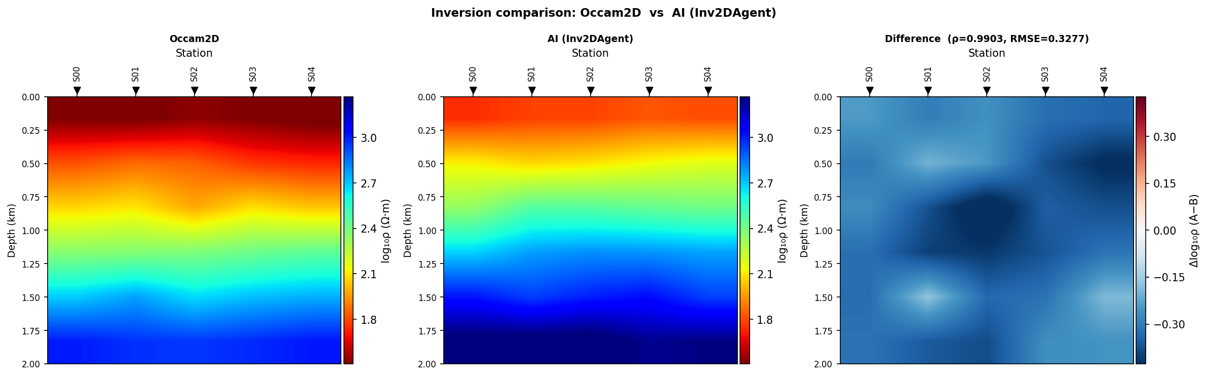
Side-by-side Occam2D and AI resistivity sections with their log10-resistivity difference. — Model A, Model B, and their difference \(A-B\) in \(\log_{10}\rho\). The difference panel is uniformly negative here because `model_b` was constructed as `model_a` plus a constant – exactly the systematic offset RMSE captured above and correlation alone would have hidden.#

4.3.9. Typical Physics-Based Chain#

Every agent on this page fits somewhere in one lifecycle, and this is that lifecycle spelled out as a chain – the same shape AgentCoordinator builds explicitly and WorkflowOrchestratorAgent builds from a natural-language request:

MTLoaderAgent -> DataQCAgent -> StaticShiftAgent
-> PhaseAnalysisAgent -> FrequencyDecimationAgent
-> Occam2DAgent or ModEmAgent or Mare2DEMAgent
-> InversionEvaluationAgent

Use InversionComparisonAgent at the end, off to the side of this main chain, when two or more of its outputs – from different backends, correction settings, or regularization choices – need to be compared and documented rather than only evaluated on their own.