
6.2.7. ModEM#
pycsamt.models.modem is the ModEM integration layer in pyCSAMT v2. It
does not reimplement the ModEM solver. Instead, it gives Python objects for
preparing ModEM input files, checking native file types, launching an external
ModEM executable, loading completed runs, and plotting the results.
ModEM projects are file-oriented. A reproducible run is normally defined by an observed data file, an initial model file, an inversion-control file, and, for 3-D inversions, a covariance file. The solver then produces iteration models, predicted responses, and logs. pyCSAMT keeps those files explicit so a project can move between Python, command-line ModEM, and archived native file folders without losing provenance.
6.2.7.1. When To Use ModEM#
Use ModEM when the survey, interpretation target, or legacy project requires a native ModEM workflow.
Good ModEM candidates include:
MT or AMT surveys with stations distributed over an area, not only one line;
geological settings where off-profile structure is expected to affect the response;
projects that need 3-D inversion, covariance masks, or region-specific smoothing;
existing ModEM projects that pyCSAMT should validate, plot, or archive;
forward-response checks against a known ModEM model;
backend-neutral pyCSAMT inversion workflows where the numerical solver is an external ModEM executable.
For simple 2-D CSAMT profile inversions, Occam2D may be more direct. For large 3-D MT or AMT modelling, ModEM is usually the more appropriate native backend.
6.2.7.2. Dimensionality#
ModEM supports both 2-D and 3-D modes in pyCSAMT. The mode controls the model class, file set, executable name, and whether a covariance file is expected.
Mode |
Main model object |
Native model file |
Typical use |
|---|---|---|---|
|
|
Profile inversion, TE/TM or selected impedance components. |
|
|
|
Area surveys, full impedance tensors, and 3-D covariance control. |
Mode |
Default executable |
Covariance file |
Default builder output |
|---|---|---|---|
|
|
Not created by |
|
|
|
Created from the 3-D model grid |
|
6.2.7.3. Package Map#
The public ModEM API is grouped around native file roles.
Object or function group |
Role |
|---|---|
Stores data settings, dimensionality, grid controls, covariance controls, inversion-control values, file names, executable names, and MPI settings. |
|
Builds a consistent ModEM input directory from EDI-like station objects
or a populated |
|
Reads, writes, and builds ModEM observed or predicted data files. |
|
Reads, writes, and creates 2-D ModEM resistivity models. |
|
Reads, writes, and creates 3-D ModEM resistivity models. |
|
Represents 3-D smoothing coefficients, region masks, and smoothing exceptions. |
|
Reads and writes the |
|
Assembles and runs external ModEM inversion or forward commands. |
|
Scans a run directory and loads models, responses, covariance, control, and logs. |
|
Parses iteration number, RMS, objective value, model norm, lambda, and alpha from a ModEM log. |
|
|
Matplotlib diagnostics for convergence, model inspection, station responses, and pseudo-sections. |
|
Vertical curtain through a 3-D model along a profile line, with
optional terrain and station-name context. Not re-exported at the
package top level; import it from |
|
Identify ModEM data, model, covariance, control, and log files before reading or routing them. |
|
Convert older impedance, Mackie, MeshTools, and interpolation-oriented file formats. |
6.2.7.4. Configuration#
Most workflows start with ModEmConfig. The same
configuration object is passed to the builder, runner, control file, model
factory, covariance factory, and result loader.
 1>>> from pycsamt.models.modem import ModEmConfig
 2
 3>>> cfg = ModEmConfig(
 4...     mode="3d",
 5...     component_type="Full_Impedance",
 6...     error_floor_z=0.05,
 7...     initial_rho=100.0,
 8...     nx=24,
 9...     ny=24,
10...     nz=36,
11...     cell_size_h=500.0,
12...     cell_size_v_top=10.0,
13...     depth_scale=1.18,
14...     n_padding_xy=8,
15...     smooth_x=0.2,
16...     smooth_y=0.2,
17...     smooth_z=0.1,
18...     n_smooth_iter=2,
19...     max_iterations=80,
20...     target_rms=1.05,
21...     binary_3d="Mod3DMT",
22...     use_mpi=True,
23...     n_procs=16,
24... )
25
26>>> cfg.write_template("runs/modem_3d_v01/modem_config.yml")
The template can be edited and loaded again:
1>>> from pycsamt.models.modem import ModEmConfig
2
3>>> cfg = ModEmConfig.from_file("runs/modem_3d_v01/modem_config.yml", strict=True)
4>>> print(cfg.mode, cfg.binary_name)
53d Mod3DMT
Use a .py, .json, .yml, or .yaml suffix – the same formats
pycsamt.models.config_io supports everywhere else in pyCSAMT. A
.ini suffix is silently accepted by write_template (it falls back to
the default .py writer while keeping the .ini name), but
from_file then rejects that same file, because it dispatches strictly on
the file extension: ValueError: Unsupported config suffix. Use .py, .json,
.yml, or .yaml. Pick a real suffix from the start.
Important settings are grouped as follows.
Setting group |
Main fields |
|---|---|
Dimensionality |
|
Data block |
|
2-D grid |
|
3-D grid |
|
Regularization |
|
Nonlinear inversion |
|
File names |
|
Execution |
|
The nonlinear-inversion group drives the same NLCG search that writes
Modular_NLCG files: initial_lambda and lambda_divisor schedule the
trade-off parameter, initial_alpha sets the first line-search step, and
rms_diff_tol/lambda_exit decide when the search has stalled rather
than converged.
6.2.7.5. Native Files#
A ModEM run folder should be understandable without Python. pyCSAMT therefore writes and reads the same native file roles that the executable uses.
File role |
Python object |
Notes |
|---|---|---|
Observed data |
|
ASCII data blocks grouped by component type. Built from EDI-like station objects or read from existing ModEM files. |
2-D model |
|
|
3-D model |
|
|
Covariance |
|
3-D earth-only smoothing file. It stores smoothing arrays, exceptions, and integer masks. |
Control |
|
|
Log |
|
Parsed convergence history from ModEM text logs. |
Predicted data |
|
Loaded by |
Validate files before routing them into a workflow. detect_file_type
returns a plain string, not an object with a .value attribute – compare
it against ModEmFileType constants or other strings directly:
 1>>> from pathlib import Path
 2
 3>>> from pycsamt.models.modem import ModEmFileType, detect_file_type
 4
 5>>> sample_dir = Path("data/modem/willy_27freq_watex_line02_sample")
 6>>> for path in sorted(sample_dir.iterdir()):
 7...     kind = detect_file_type(path)
 8...     if kind != ModEmFileType.UNKNOWN:
 9...         print(path.name, kind)
1027-freq-run-watex01.cov covariance
1127-freq-run-watex01.dat data
1227-freq-run-watex01.rho model_3d
13inv.ctrl control
14Modular_NLCG.log log
15Modular_NLCG_000.dat data
16Modular_NLCG_000.rho model_3d
17Modular_NLCG_030.dat data
18Modular_NLCG_030.res data
19Modular_NLCG_030.rho model_3d
20Modular_NLCG_073.dat data
21Modular_NLCG_073.res data
22Modular_NLCG_073.rho model_3d
run.slurm, fwd.ctrl, fort.2000, CSUr2.err, and README.txt
are correctly left out – they are real files in this bundled sample
directory, just not ones detect_file_type claims to recognize.
.res residual files are classified as data alongside the .dat
files they pair with.
6.2.7.6. Data Files And Components#
ModEmData stores observed or predicted response
rows. pyCSAMT can read existing ModEM data files or build new ones from
station objects.
When building from EDI-like objects, each station should provide:
a station name;
station coordinates or latitude/longitude/elevation metadata;
positive frequencies;
complex impedance values shaped like
(n_frequency, 2, 2);impedance errors or uncertainty estimates.
The configuration selects which response components are written. Supported
component_type values include:
|
Components written |
|---|---|
|
|
|
|
|
|
|
|
|
|
|
|
|
|
ModEmData.from_edi accepts the same kind of survey source as the Occam2D
builder – a Sites container, not a bare path string:
 1>>> from pycsamt.models.modem import ModEmConfig, ModEmData
 2>>> from pycsamt.site import Sites
 3
 4>>> sites = Sites.from_any("data/AMT/WILLY_DATA/L18PLT")
 5
 6>>> cfg = ModEmConfig(
 7...     mode="3d",
 8...     component_type="Off_Diagonal_Impedance",
 9...     error_floor_z=0.05,
10...     freq_min=1e-3,
11...     freq_max=1e3,
12... )
13
14>>> data = ModEmData.from_edi(sites, config=cfg)
15>>> data.write("runs/modem_3d_v01/native/ModEMData.dat")
16
17>>> print(data.n_sites, data.n_periods, data.component_types)
1828 53 ['Off_Diagonal_Impedance']
Important
ModEM data files depend on consistent local coordinates. The pyCSAMT writer
stores local x, y, and z coordinates used by the model builder.
Confirm projection, station order, and units before inversion. Do not mix
metres, kilometres, and geographic degrees inside the same run folder.
6.2.7.7. Build A 3-D Input Set#
InputBuilder creates the standard 3-D input
set: observed data, starting model, covariance, and control file.
 1>>> from pathlib import Path
 2
 3>>> from pycsamt.models.modem import InputBuilder, ModEmConfig
 4>>> from pycsamt.site import Sites
 5
 6>>> sites = Sites.from_any("data/AMT/WILLY_DATA/L18PLT")
 7
 8>>> workdir = Path("runs/modem_3d_v01/native")
 9>>> cfg = ModEmConfig(
10...     mode="3d",
11...     component_type="Full_Impedance",
12...     initial_rho=100.0,
13...     nx=28,
14...     ny=28,
15...     nz=38,
16...     n_airlayers=5,
17...     cell_size_h=500.0,
18...     cell_size_v_top=10.0,
19...     depth_scale=1.18,
20...     n_padding_xy=8,
21...     smooth_x=0.2,
22...     smooth_y=0.2,
23...     smooth_z=0.1,
24...     n_smooth_iter=2,
25... )
26
27>>> builder = InputBuilder(config=cfg)
28>>> files = builder.build(
29...     sites,
30...     workdir=workdir,
31...     data_filename=cfg.data_file,
32...     model_filename="m0.ws",
33...     cov_filename=cfg.covariance_file,
34...     ctrl_filename=cfg.control_file,
35... )
36
37>>> for role, path in sorted(files.items()):
38...     print(role, path.name)
39control ModEM.inv
40covariance ModEM.cov
41data ModEMData.dat
42model m0.ws
The returned mapping contains data, model, covariance, and
control. The builder also keeps the populated objects on
builder.data, builder.model, builder.covariance, and
builder.control for inspection.
6.2.7.8. Build A 2-D Input Set#
The 2-D builder path writes data, a 2-D half-space model, and a control file. It does not create a 3-D covariance file.
 1>>> from pycsamt.models.modem import InputBuilder, ModEmConfig
 2
 3>>> cfg = ModEmConfig(
 4...     mode="2d",
 5...     component_type="TE_Impedance",
 6...     initial_rho=100.0,
 7...     nx_2d=120,
 8...     nz_2d=60,
 9...     n_airlayers_2d=5,
10...     cell_size_h_2d=100.0,
11...     cell_size_v_top_2d=10.0,
12...     depth_scale_2d=1.18,
13...     n_padding_x_2d=8,
14...     max_iterations=60,
15... )
16
17>>> files = InputBuilder(config=cfg).build(
18...     sites,
19...     workdir="runs/modem_2d_v01/native",
20...     data_filename="ModEMData.dat",
21...     model_filename="m0.rho",
22...     ctrl_filename="ModEM.inv",
23... )
24
25>>> print(sorted(files))
26['control', 'data', 'model']
27>>> assert "covariance" not in files
6.2.7.9. Build From Existing Data#
Use build_from_data when the observed data object has already been read,
filtered, or edited. In this mode the builder creates the model, covariance
when needed, and control file. The caller is responsible for writing the data
file itself.
 1>>> from pycsamt.models.modem import InputBuilder, ModEmConfig, ModEmData
 2
 3>>> cfg = ModEmConfig(mode="3d")
 4>>> data = ModEmData.read(
 5...     "data/modem/willy_27freq_watex_line02_sample/27-freq-run-watex01.dat"
 6... )
 7>>> data.write("runs/modem_3d_v02/native/ModEMData.dat")
 8
 9>>> files = InputBuilder(config=cfg).build_from_data(
10...     data,
11...     workdir="runs/modem_3d_v02/native",
12...     model_filename="m0.ws",
13...     cov_filename="ModEM.cov",
14...     ctrl_filename="ModEM.inv",
15... )
16>>> print(sorted(files))
17['control', 'covariance', 'model']
6.2.7.10. Models#
The model objects store cell widths and resistivity values. Internally,
resistivity is stored in natural-log units because ModEM solves for log
resistivity. The rho_linear property returns resistivity in linear
ohm m units for plotting and interpretation.
Create and inspect a 3-D starting model:
 1>>> from pycsamt.models.modem import ModEmData, ModEmModel3D, ModEmConfig
 2
 3>>> cfg = ModEmConfig(mode="3d", initial_rho=100.0)
 4>>> data = ModEmData.read("runs/modem_3d_v01/native/ModEMData.dat")
 5
 6>>> model = ModEmModel3D.halfspace(data, config=cfg)
 7>>> model.write("runs/modem_3d_v01/native/m0.ws")
 8
 9>>> print(model.shape)
10(35, 30, 40)
11>>> print(model.n_air)
125
13>>> print(model.rho_linear.min(), model.rho_linear.max())
14100.00000000000004 999999999999.999
The maximum is not a bug: air cells are assigned an enormous placeholder
resistivity (\(\sim 10^{12}\,\Omega\cdot\mathrm{m}\)) rather than
\(\infty\), so rho_linear.max() on a fresh half-space always reports
the air value, not anything about the earth model.
Create and inspect a 2-D starting model:
 1>>> from pycsamt.models.modem import ModEmData, ModEmModel2D, ModEmConfig
 2
 3>>> cfg = ModEmConfig(mode="2d", initial_rho=100.0)
 4>>> data = ModEmData.read("runs/modem_2d_v01/native/ModEMData.dat")
 5
 6>>> model = ModEmModel2D.halfspace(data, config=cfg)
 7>>> model.write("runs/modem_2d_v01/native/m0.rho")
 8
 9>>> print(model.nx, model.nz)
1042 55
11>>> print(model.x_nodes[-1], model.z_nodes[-1])
1250861.204999999994 455021.9075001069
The half-space factories are intentionally conservative. They are useful for a first run, but a production inversion usually deserves a deliberate mesh review: station spacing, padding, first-layer thickness, air layers, expected skin depths, and target depth all matter.
6.2.7.11. Covariance#
The covariance file is central to 3-D ModEM interpretation. It controls the model regularization term through smoothing coefficients and integer masks. pyCSAMT creates a uniform active earth region by default, then lets advanced users edit masks and exceptions before writing the file.
1>>> from pycsamt.models.modem import ModEmCovariance
2
3>>> cov = ModEmCovariance.from_model(model, config=cfg)
4>>> cov.exceptions.append((1, 2, 0.0))  # turn off smoothing across two regions
5>>> cov.write("runs/modem_3d_v01/native/ModEM.cov")
Mask values follow the ModEM convention:
0is reserved for air;9is reserved for ocean;1through8are user-defined earth regions.
ModEmCovariance.from_model excludes air layers from the covariance grid.
model.shape is (nz, ny, nx) – for the 3-D starting model built above
that is (35, 30, 40), so model.nz is 35, not the nx=40 most
readers’ eyes land on first. With model.n_air=5, the covariance carries
model.nz - model.n_air = 30 layers.
6.2.7.12. Control Files#
ModEmControl stores the nonlinear inversion
settings written to the .inv file.
 1>>> from pycsamt.models.modem import ModEmConfig, ModEmControl
 2
 3>>> cfg = ModEmConfig(
 4...     output_stem="ModEM_out",
 5...     initial_lambda=10.0,
 6...     lambda_divisor=100.0,
 7...     initial_alpha=10.0,
 8...     rms_diff_tol=5e-4,
 9...     target_rms=1.05,
10...     lambda_exit=1e-4,
11...     max_iterations=100,
12... )
13
14>>> control = ModEmControl.from_config(cfg)
15>>> control.write("runs/modem_3d_v01/native/ModEM.inv")
The control file does not replace data-quality assessment. A low target RMS is meaningful only when uncertainty floors, component selection, and bad-period masking are realistic.
6.2.7.13. Run ModEM#
ModEmRunner assembles the external command and
can execute it with subprocess.run(). The executable is resolved from
PATH or from the run directory and local _source/2D or _source/3D
subdirectories.
ModEM is not a Python dependency and pyCSAMT does not ship a pre-compiled executable. Build it first by following ModEM. For the standard serial 3-D build, the short form is:
pycsamt build modem3d --auto-install
After a successful build, configure the runner with the executable path that
the build command prints. The following finds that executable in pyCSAMT’s
ModEM source tree, works with editable and regular installations, and handles
the Windows .exe suffix:
Always inspect the command first:
 1>>> import os
 2>>> from pathlib import Path
 3
 4>>> import pycsamt.models.modem as modem
 5>>> from pycsamt.models.modem import ModEmConfig, ModEmRunner
 6
 7>>> binary_name = "Mod3DMT.exe" if os.name == "nt" else "Mod3DMT"
 8>>> binary = Path(modem.__file__).resolve().parent / "_source" / "3D" / binary_name
 9>>> if not binary.is_file():
10...     raise FileNotFoundError(
11...         f"{binary} was not built; see the ModEM compilation guide"
12...     )
13
14>>> cfg = ModEmConfig(
15...     mode="3d",
16...     binary_3d=str(binary),
17...     use_mpi=False,
18... )
19
20>>> runner = ModEmRunner("runs/modem_3d_v01/native", config=cfg)
21>>> command = runner.command(
22...     "m0.ws",
23...     "ModEMData.dat",
24...     "ModEM.inv",
25...     covariance="ModEM.cov",
26... )
27>>> print(command)
28...Mod3DMT -I NLCG m0.ws ModEMData.dat ModEM.inv ModEM.cov
Run the inversion only after file paths, executable names, and MPI settings are correct:
1result = runner.run(
2    "m0.ws",
3    "ModEMData.dat",
4    "ModEM.inv",
5    covariance="ModEM.cov",
6    timeout=24 * 3600,
7    load_result=True,
8)
The code block is intentionally not a doctest: it launches the external
solver and may run for hours. When load_result=True, a successful process
returns an InversionResult populated from the
run directory.
For MPI, compile the MPI variant as described in ModEM,
then set use_mpi=True, n_procs to the desired process count, and
mpi_command to the launcher available on the system. Do not enable MPI
for the standard serial build.
For a forward response check, call run_forward:
1>>> # runner.run_forward(
2>>> #     "m0.ws",
3>>> #     "ModEMData.dat",
4>>> #     timeout=3600,
5>>> #     load_result=False,
6>>> # )
Warning
The runner is a subprocess wrapper around an external executable. It cannot make a physically poor mesh, incorrect component selection, or inconsistent coordinate system valid. Treat the generated command as a reproducibility aid, not as a scientific approval stamp.
6.2.7.14. Load Results#
InversionResult scans a completed run directory
and loads what it finds: logs, controls, covariance, data files, and iteration
models.
None of the sections above actually launched ModEM – there is no compiled
binary in a documentation-build environment. From here on, the examples load
a genuinely finished run instead: the compact willy_27freq_watex_line02_sample
bundled with pyCSAMT, built specifically for documentation and gallery use
from a real 3-D MT inversion (see its README.txt for provenance). It keeps
only three representative iteration snapshots – 0, 30, and 73 – rather than
every step the production run wrote.
 1>>> from pycsamt.models.modem import InversionResult
 2
 3>>> result = InversionResult("data/modem/willy_27freq_watex_line02_sample")
 4
 5>>> print(result.mode, result.n_iter)
 63d 74
 7>>> print(round(result.final_rms, 4), round(result.best_rms, 4))
 83.0572 3.0572
 9>>> print(sorted(result.models))
10['iter_0000', 'iter_0030', 'iter_0073']
11
12>>> final_model = result.model_final
13>>> observed = result.data_obs
14>>> predicted = result.data_pred
15>>> print(final_model.shape, observed.n_sites)
16(41, 50, 288) 125
result.n_iter (74) counts iterations recorded in the log, not how many
.rho snapshots are physically present – only 3 of those 74 models are
bundled. final_rms equals best_rms here only because this particular
run’s RMS happened to keep falling, slowly, all the way to iteration 73; nothing
in the loader guarantees that in general, which is exactly why both numbers
exist separately. An RMS of 3.06 is well above the target of 1.0 – this run
did not converge, and every plot in the next two sections should be read with
that in mind.
The result loader recognizes common ModEM output naming patterns, including
numbered Modular_NLCG products. The lowest numbered response can be used
as an observed-data fallback and the highest numbered response can be used as
the predicted response when explicit filenames are not available.
6.2.7.15. Log Diagnostics#
Use ModEmLog when the convergence history is
the primary diagnostic.
 1>>> from pycsamt.models.modem import ModEmLog
 2
 3>>> log = ModEmLog.read(
 4...     "data/modem/willy_27freq_watex_line02_sample/Modular_NLCG.log"
 5... )
 6
 7>>> print(log.n_iter, round(log.final_rms, 4), log.best_iter)
 874 3.0572 73
 9>>> print(round(log.rms[0], 4), round(log.rms[-1], 4))
103.5197 3.0572
11>>> print(log.lagrange[:5])
12[20. 20. 20. 20. 20.]
Review more than the final RMS. Sudden RMS stalls, unstable lambda changes,
or a best iteration far earlier than the final iteration can indicate
overfitting, inconsistent errors, or a regularization setting that should be
revisited. Here best_iter (73) is the final iteration, which is the
unremarkable case; a best iteration well before the end is the pattern
actually worth stopping for.
6.2.7.16. Plotting#
The ModEM plotters operate on
InversionResult objects and return Matplotlib
figures. All of the figures below come from the same
willy_27freq_watex_line02_sample result loaded above.
 1>>> from pathlib import Path
 2
 3>>> from pycsamt.models.modem import PlotMisfit, PlotModel3D, PlotPseudo, PlotResponse
 4
 5>>> Path("runs/modem_3d_v01/figures").mkdir(parents=True, exist_ok=True)
 6
 7>>> fig = PlotMisfit(result=result).plot()
 8>>> fig.savefig("runs/modem_3d_v01/figures/rms.png", dpi=200)
 9
10>>> fig = PlotModel3D(
11...     result=result,
12...     depths=[500, 1000, 2000, 4000],
13...     rho_min=1.0,
14...     rho_max=1000.0,
15... ).plot()
16>>> fig.savefig("runs/modem_3d_v01/figures/model_slices.png", dpi=200)
17
18>>> stations = list(result.data_obs.site_names)[:2]
19>>> fig = PlotResponse(result=result, stations=stations, max_stations=2).plot()
20>>> fig.savefig("runs/modem_3d_v01/figures/responses.png", dpi=200)
21
22>>> fig = PlotPseudo(result=result, component="ZXY").plot()
23>>> fig.savefig("runs/modem_3d_v01/figures/pseudo_zxy.png", dpi=200)
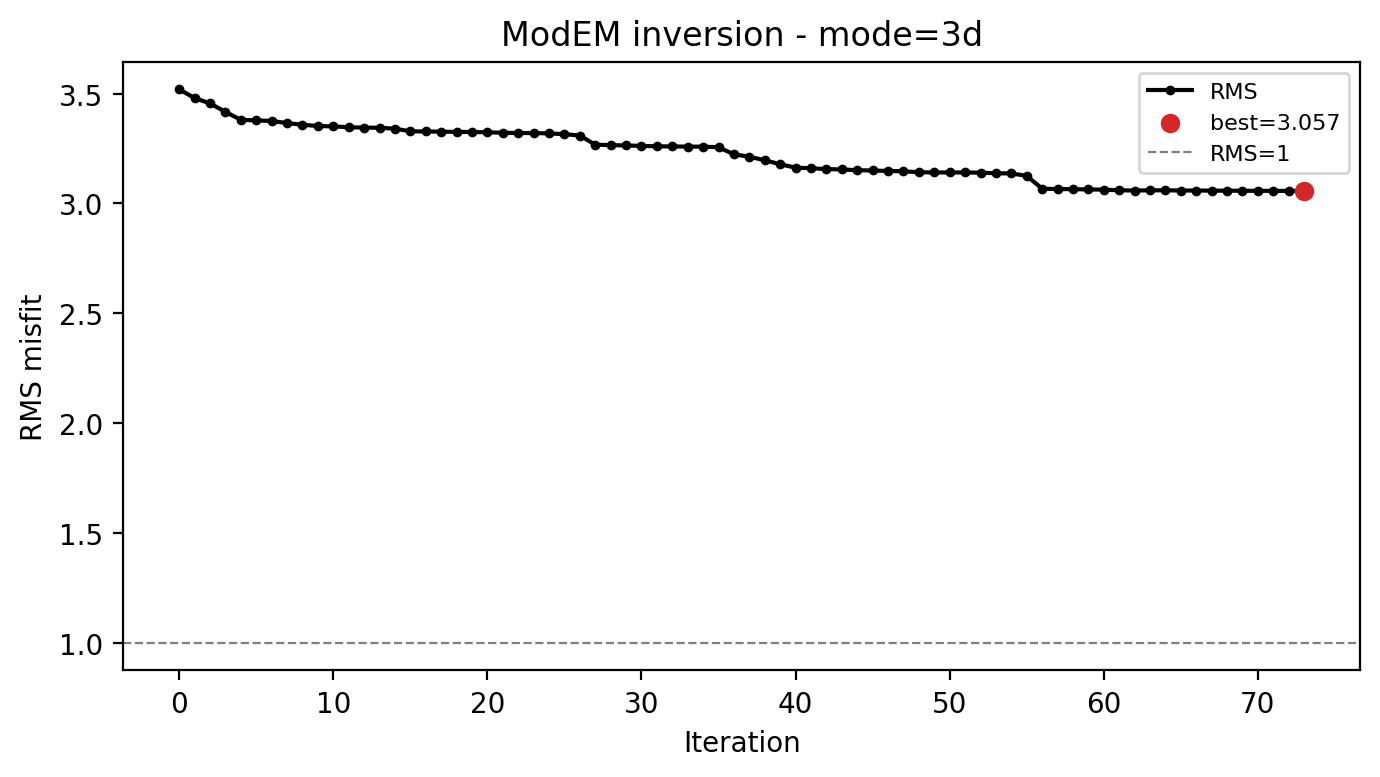
RMS drops from 3.52 to 3.06 over 74 iterations but never gets close to the
dashed target line at 1.0. Two long flat stretches (iterations 5-25 and
40-55) suggest the search was making very slow progress well before it
stopped – worth checking against log.lagrange and the control file’s
rms_diff_tol before trusting the final model.#
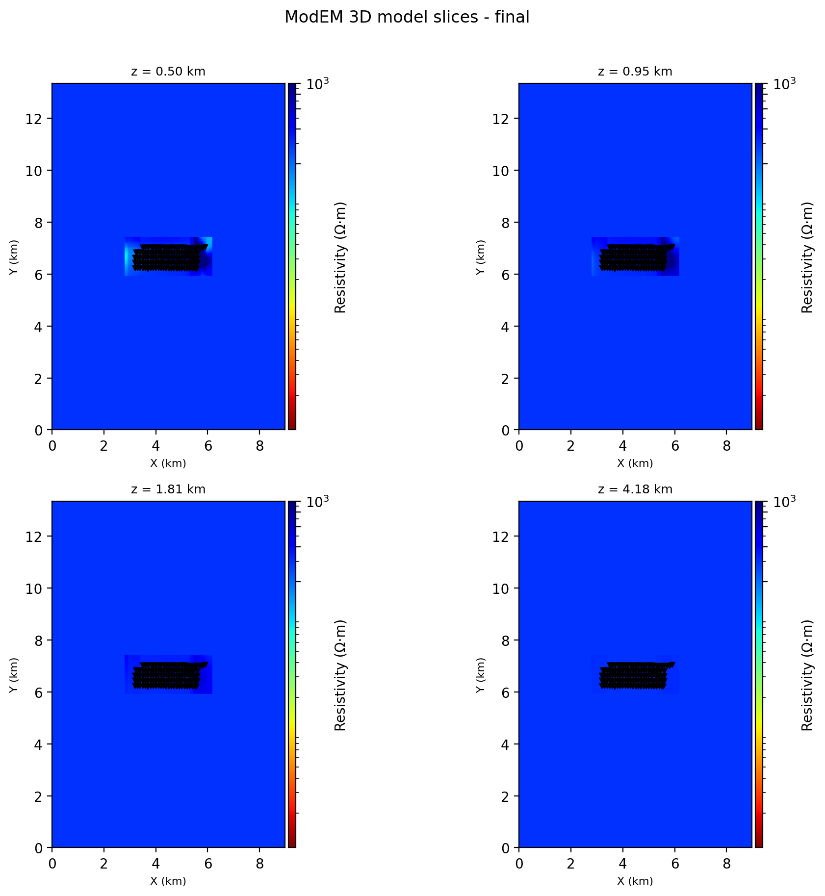
Four depth slices through model_final, all essentially uniform at
this color scale. That is not a plotting mistake – it is what a model
looks like after an inversion that stalled at RMS 3.06: with the data
still fit this poorly, the regularization has not been pushed hard enough
by the data misfit to build much lateral contrast. A suspiciously
featureless model slice is a reason to check the convergence plot, not a
reason to conclude the subsurface is uniform.#
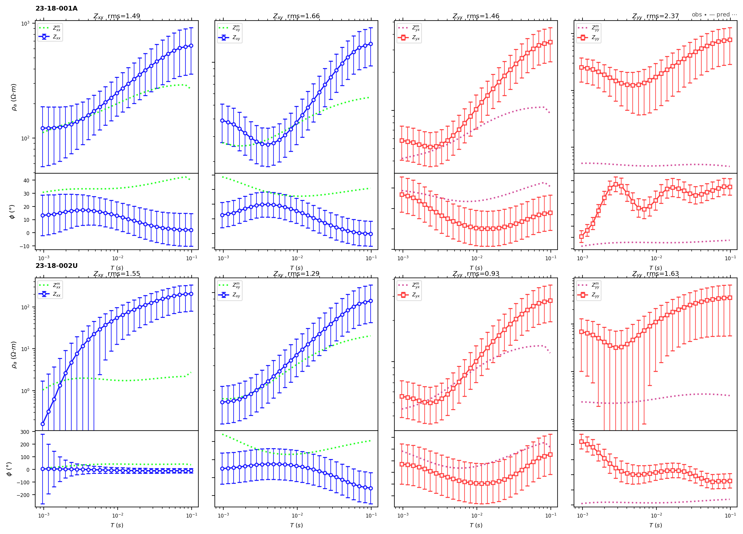
Station-level detail behind that RMS 3.06: for both stations, the predicted curves (dotted) track the observed apparent resistivity (solid, with error bars) at short period but drift away at long period, and the phase panels barely follow the observed trend at all in three of the four off-diagonal components. This is what “did not converge” looks like at the response level, not just as a single summary number.#
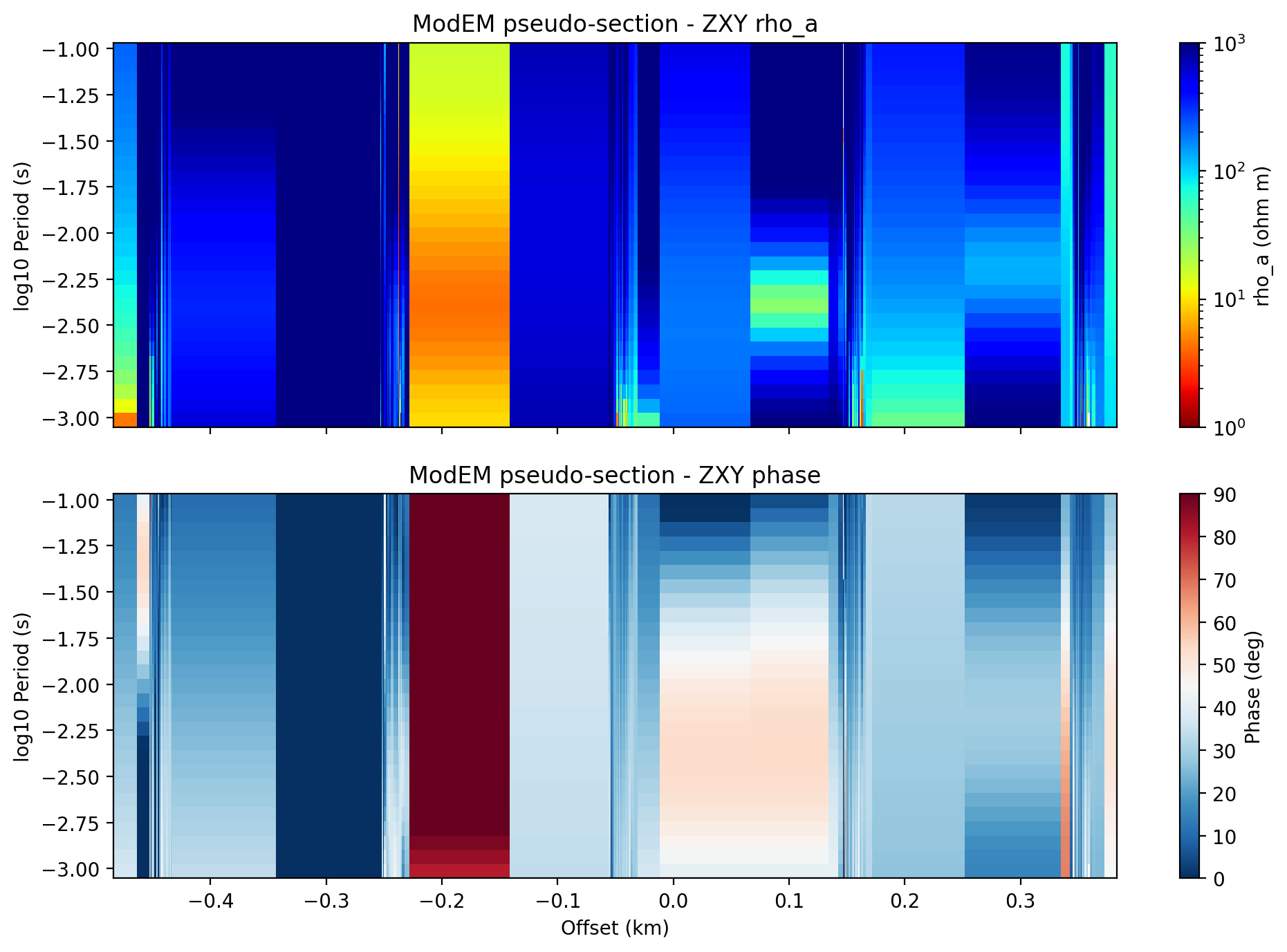
component="ZXY" pseudo-section over all 125 stations. The banded
structure – alternating resistive and conductive columns rather than a
smooth lateral trend – reflects that this is an areal 3-D deployment
sampled along an arbitrary station ordering, not a single profile line;
compare with Occam2D’s pseudosection, which is genuinely
profile-ordered by chainage.#
For 2-D results, use pycsamt.models.modem.PlotModel2D the same way:
1>>> from pycsamt.models.modem import InversionResult, PlotModel2D
2
3>>> result_2d = InversionResult("runs/modem_2d_v01/native")
4>>> fig = PlotModel2D(result=result_2d, depth_max=5000.0).plot()
5>>> fig.savefig("runs/modem_2d_v01/figures/model_section.png", dpi=200)
No finished 2-D ModEM sample ships with pyCSAMT, so this one is shown without
a captured figure – runs/modem_2d_v01/native here is the half-space
starting model built earlier, not a converged result.
6.2.7.17. Geo-Referenced Depth Maps#
PlotModel3D draws depth slices in model-grid coordinates.
PlotDepthMap (import it from pycsamt.models.modem.plot) draws the
same slices as geographic maps: decimal-degree axes, station markers in
their true positions, and – by default – a crop to the station
footprint rather than the full padded mesh. The remaining examples use
the bundled 21-station Broken Hill MT survey and its converged 3-D
model (data/MT/broken-hill; see that folder’s README.md for the
data source and citation), because it is areal, well constrained, and
geo-referenced.
 1>>> from pycsamt.models.modem import InversionResult
 2>>> from pycsamt.models.modem.plot import PlotDepthMap
 3
 4>>> bh = InversionResult("data/MT/broken-hill/final-models")
 5
 6>>> fig = PlotDepthMap(
 7...     bh,
 8...     depths={"(a) 1 km": 1000, "(b) 2 km": 2000,
 9...             "(c) 3 km": 3000, "(d) 5 km": 5000},
10...     origin_lat=-31.95556,
11...     origin_lon=141.53481,
12...     rho_range=(1, 10000),
13...     mask_outside_hull=True,
14...     contours=[1000],
15...     scalebar=True,
16...     north_arrow=True,
17...     title="Broken Hill ModEM -- resistivity depth slices",
18... ).plot()
19>>> fig.savefig("bh_depthmap.png", dpi=200, bbox_inches="tight")
The ModEM data file reduces longitude by 100 degrees (the Broken Hill
header reads 41.53481), so origin_lon is passed as the true value
141.53481. depths accepts a plain list or, as here, a
{label: depth} mapping that also sets the panel titles.
mask_outside_hull=True blanks cells beyond the station convex hull so
the figure does not imply resolution the data cannot provide;
contours=[1000] adds a single iso-resistivity line at 1000 Ω·m.
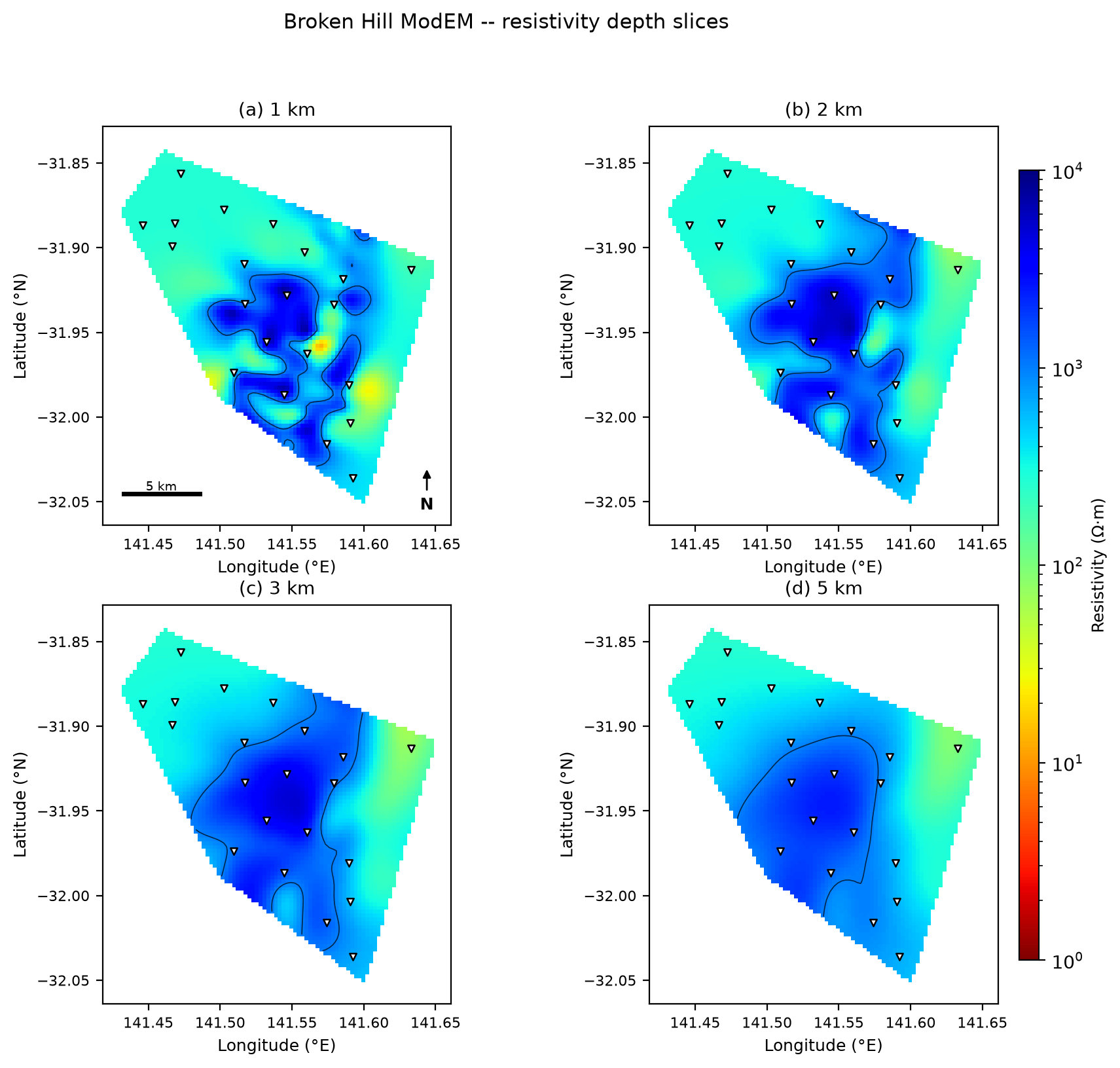
Broken Hill resistivity at 1, 2, 3 and 5 km depth. The crust is broadly resistive (blue, > 1000 Ω·m); the 1000 Ω·m contour encloses a resistive core that grows with depth. At 1 km a few small conductive patches (yellow/orange, < 30 Ω·m) sit along the station line – these coincide with the sulphide-bearing Broken Hill Group – and they fade by 3 km, consistent with shallow mineralised horizons over a resistive basement.#
The same class produces a conductance map – the depth integral of conductivity over a chosen window, \(S=\int_{z_1}^{z_2}\sigma\,dz\) in siemens – which is often the most useful single view of a mineral-system target because it collapses the vertical dimension into one number per location:
 1>>> fig = PlotDepthMap(
 2...     bh,
 3...     quantity="conductance",
 4...     conductance_window=(1000, 6000),
 5...     origin_lat=-31.95556,
 6...     origin_lon=141.53481,
 7...     render="gouraud",
 8...     cmap="magma",
 9...     norm="linear",
10...     rho_range=(10, 50),
11...     smooth_sigma=0.8,
12...     mask_outside_hull=True,
13...     station_color="white",
14...     cbar_orientation="horizontal",
15...     title="Broken Hill -- conductance, 1-6 km",
16... ).plot()
17>>> fig.savefig("bh_conductance.png", dpi=200, bbox_inches="tight")
render selects how the field is drawn: "mesh" (default) shows the
raw model cells, while "gouraud", "contourf" and "image"
interpolate between cell centres for the smooth appearance conventional
in published conductance maps. rho_range here sets the colour limits
to 10–50 S and norm="linear" keeps the scale linear over that
narrow window; station_color="white" makes the markers legible over
the dark end of magma.
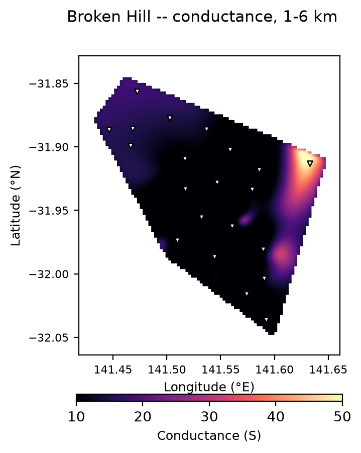
Conductance over the 1–6 km window. The interior of the survey is resistive (dark, ~10 S) and the conductive anomalies (yellow, up to ~50 S) sit on the eastern and south-eastern margin, over the mapped trace of the Broken Hill Group. A conductance map like this is what a mineral-exploration MT survey is usually reduced to before it is compared against geology and potential-field data.#
6.2.7.18. A Vertical Section Through The 3-D Model#
For 3-D results, a single vertical curtain along a profile line is often more
useful for interpretation than isolated depth slices. PlotSection (import
it from pycsamt.models.modem.plot, not the package top level) extracts one:
 1>>> from pycsamt.models.modem.plot import PlotSection
 2
 3>>> plotter = PlotSection(
 4...     result=result,
 5...     direction="NS",
 6...     profile_offset=0.0,
 7...     which="final",
 8...     depth_max=5000.0,
 9...     rho_min=1.0,
10...     rho_max=3000.0,
11...     cmap="turbo_r",
12...     show_station_names=True,
13... )
14>>> fig = plotter.plot()
15>>> ax = fig.axes[0]
16
17>>> ylo, _ = ax.get_ylim()  # (-5.696, 0.0): 0 is the surface, at the axes top
18>>> ax.set_ylim(ylo, 1.4)   # reserve headroom so labels don't collide with the title
19>>> fig.savefig("runs/modem_3d_v01/figures/section_ns.png", dpi=200)
Station-name labels are drawn starting exactly at the surface line and
growing upward, with no headroom reserved above it – without the
set_ylim adjustment they overlap the title directly. This is the same
class of matplotlib default seen in Occam2D’s rotated station labels:
nothing places text safely on its own, so the caller reserves the room.
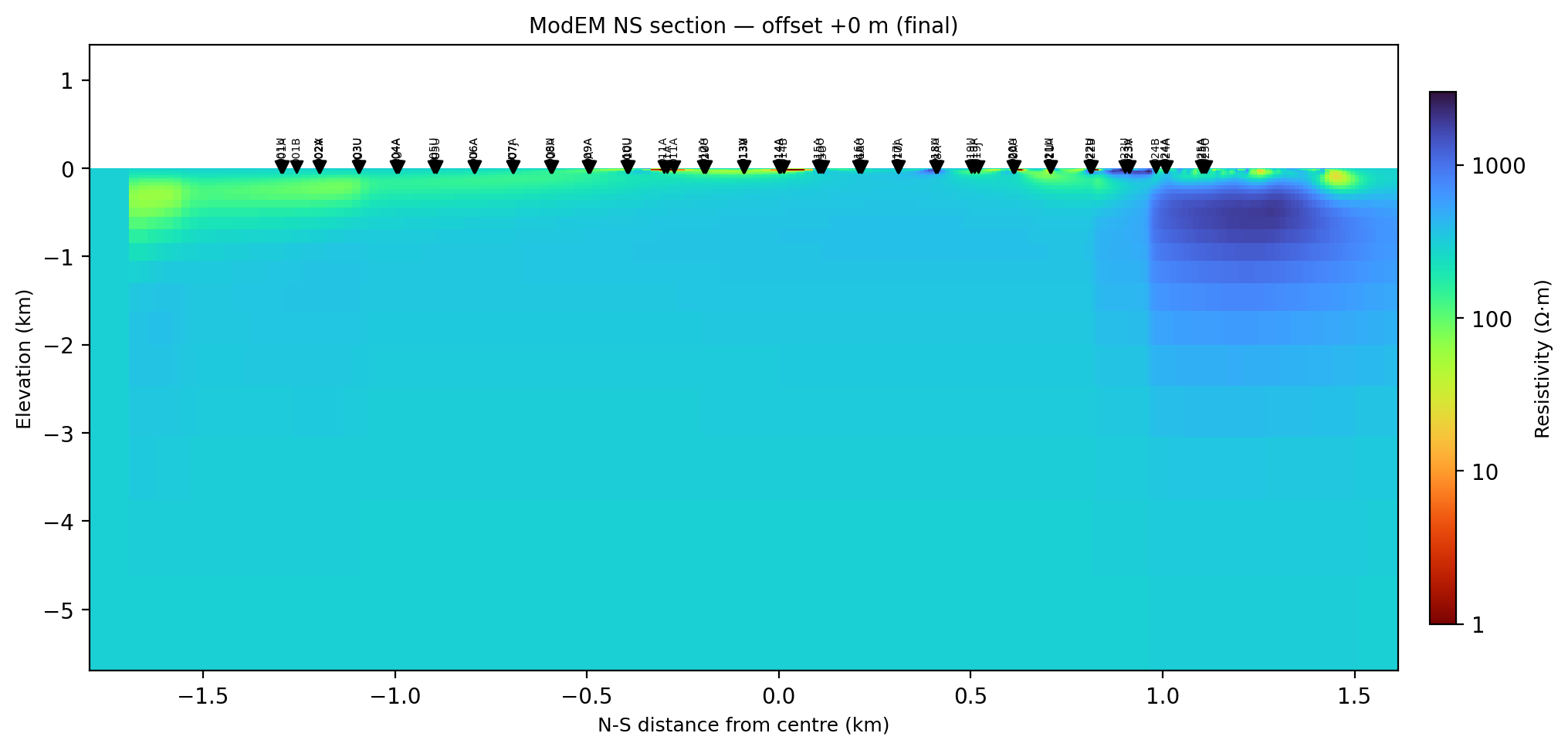
A resistive body (dark blue/purple, exceeding the 3000 ohm-m color
ceiling) sits under the stations between roughly +0.9 and +1.5 km,
confined to the top ~1.3 km – the same profile-relative signature
PlotModel3D’s depth slices above were too uniform-looking to convey.
With RMS still at 3.06, treat this as a candidate feature to re-run and
re-check, not a finished interpretation.#
The axis-aligned mode above cuts the section parallel to a mesh axis at a
fixed perpendicular offset. It works well when the mesh is only lightly
padded, but on a heavily padded 3-D grid the automatic horizontal extent
can collapse to a sliver or blow out to the full padded width. The
robust alternative is arbitrary-azimuth mode: pass start_point
and end_point as (lat, lon) with use_latlon=True and the
section follows exactly the line you specify, sampled at n_samples
points.
 1>>> bh = InversionResult("data/MT/broken-hill/final-models")
 2>>> fig = PlotSection(
 3...     result=bh,
 4...     start_point=(-31.860, 141.490),   # NW
 5...     end_point=(-32.020, 141.610),     # SE, across strike
 6...     use_latlon=True,
 7...     origin_lat=-31.95556,
 8...     origin_lon=141.53481,
 9...     n_samples=320,
10...     depth_max=8000.0,
11...     rho_min=1.0,
12...     rho_max=5000.0,
13...     show_station_names=False,
14...     station_tol=2500.0,
15...     title="Broken Hill ModEM -- section B-B' (NW -> SE)",
16... ).plot()
17>>> fig.savefig("bh_section.png", dpi=200, bbox_inches="tight")
station_tol is the maximum perpendicular distance (metres) for a
station to be projected onto the section; widen it for a sparse survey,
tighten it for a dense one. depth_max clips the featureless deep
part of the model that the shallow survey does not constrain.
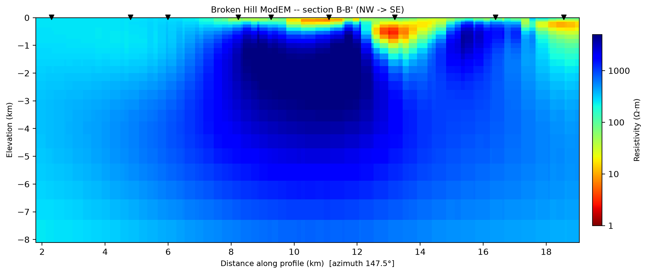
The Broken Hill model cut NW–SE across the structural grain. A resistive (> 1000 Ω·m, blue) crust is punctuated by shallow conductors (red/orange, < 10 Ω·m) confined to the top ~1.5 km – the same anomalies visible as yellow patches on the depth maps above, now resolved as discrete near-surface bodies rather than a smeared layer. Because the section is defined by geographic coordinates it can be drawn along the exact trace of a mapped geological cross-section for a direct comparison.#
6.2.7.19. Conversion And Utility Tools#
The ModEM package also exposes utility functions for existing projects and format conversion.
Utility group |
Examples |
|---|---|
Impedance files |
|
Mackie formats |
|
MeshTools export |
|
Interpolation |
|
Units and transforms |
|
skin_depth implements the same \(\delta \approx 503\sqrt{\rho T}\)
relation used throughout pyCSAMT’s skin depth diagnostics, taking
period rather than frequency:
1>>> from pycsamt.models.modem import skin_depth
2
3>>> print(round(skin_depth(period=1.0, rho=100.0), 1))
45032.9
These helpers are most useful when a project arrives with older ModEM, Mackie, or impedance-list files and pyCSAMT is being used as a bridge into a clean v2 run directory.
6.2.7.20. Backend-Neutral Workflows#
The native objects above are the most explicit way to work with ModEM. pyCSAMT also exposes ModEM through the backend-neutral inversion interface.
 1>>> from pycsamt.inversion import InversionConfig, InversionWorkflow
 2>>> from pycsamt.site import Sites
 3
 4>>> inv_cfg = InversionConfig(
 5...     method="mt",
 6...     dimension="3d",
 7...     backend="modem",
 8...     data="data/AMT/WILLY_DATA/L18PLT",
 9...     workdir="runs/modem_3d_backend_neutral/native",
10...     run_external=False,
11...     backend_options={
12...         "config": {
13...             "component_type": "Full_Impedance",
14...             "initial_rho": 100.0,
15...             "binary_3d": "Mod3DMT",
16...             "use_mpi": True,
17...             "n_procs": 16,
18...         },
19...     },
20... )
21>>> workflow = InversionWorkflow(inv_cfg)
22>>> sites = Sites.from_any(inv_cfg.data)
23>>> outcome = workflow.run(data=sites)
24>>> print(outcome.status, outcome.rms)
25loaded nan
status="loaded" here does not mean an inversion ran – rms is
nan right next to it. The Occam2D backend only reports "loaded"
once it has reconstructed a real resistivity grid from an actual iteration
file; the ModEM backend’s loaded-check is coarser (`` “has anything
InversionResult can parse” ), and a just-built starting model already
satisfies that after ``InputBuilder runs, whether or not ModEM ever
executed. Check rms – or, better, result.n_iter – before treating
status="loaded" from this backend as evidence of a finished run.
With run_external=False, the backend prepares or validates the run folder
and reports the command that would be executed. Set run_external=True only
when the external ModEM executable is installed and the run directory has been
reviewed.
6.2.7.21. Recommended Run Layout#
A stable ModEM project layout separates native inputs, figures, and notes:
 1runs/
 2  modem_3d_v01/
 3    README.md
 4    config/
 5      modem_config.yml
 6    native/
 7      ModEMData.dat
 8      m0.ws
 9      ModEM.cov
10      ModEM.inv
11      Modular_NLCG.log
12      Modular_NLCG_030.rho
13      Modular_NLCG_030.dat
14    figures/
15      rms.png
16      model_slices.png
17      responses.png
18      section_ns.png
19    exports/
20      final_model.vtk
Keep hand-edited files under version control when possible. Large model outputs and response grids can be archived separately if repository size is a concern.
6.2.7.22. Pre-Run Checklist#
Before starting a ModEM inversion, verify:
station coordinates use one local coordinate system and metre units;
periods and frequencies are in the intended range;
impedance sign convention and units match the executable expectation;
component selection is appropriate for the survey dimensionality;
error floors are realistic and bad periods have been removed or masked;
horizontal cell size reflects station spacing and target resolution;
vertical first-layer thickness and depth growth resolve shallow structure;
padding extends far enough from the station footprint;
air layers and ocean or inactive masks are correct;
covariance smoothing values and exceptions are scientifically justified;
the dry-run command points to the intended executable and files;
MPI process count matches the machine and executable build.
6.2.7.23. Post-Run Checklist#
After a run finishes, review:
RMS history and best iteration, not only final RMS;
response fits by station, period, and component;
residual concentration around specific stations or period bands;
model updates near boundaries, air layers, and padding cells;
sensitivity of interpretation to error floors and covariance settings;
consistency between final model features and known geology;
reproducibility of the run directory, configuration, command, and code version.
6.2.7.24. Common Mistakes#
The command is ready but the executable cannot be found.Check
binary_2dorbinary_3dinModEmConfig. The runner searchesPATH, the working directory, and local_sourcefolders.The 3-D run is missing a covariance file.Build the input set with
mode="3d"or createModEmCovariancefrom the 3-D model and pass it to the runner.The model loads but plotted station positions look wrong.Recheck coordinate origin, projection, and units before trusting any response or model diagnostics.
The RMS is low but the model has unrealistic detail.Inspect uncertainty floors, removed periods, smoothing values, covariance masks, and response residuals. A visually detailed model is not necessarily better constrained.
The result loader did not find a predicted response.Confirm the output stem in the control file and inspect the run directory for numbered
Modular_NLCGresponse files.A config template written with a ".ini" suffix will not load back.write_templateaccepts the path anyway and writes Python-format content into it;from_filethen rejects the same file because it reads the extension, not the content. Use.py,.json,.yml, or.yaml.The backend-neutral result says "loaded" but nothing was ever run.Check
result.rmstoo. The ModEM backend reports"loaded"as soon asInversionResultcan parse anything in the workdir, which includes a freshly built starting model – it is not the stronger guarantee the Occam2D backend gives for the same status string.
6.2.7.25. Next Steps#
Prepare A ModEM Inversion walks through preparing a real 3-D ModEM run end to end, including horizontal and vertical mesh design.
Compiling the External Solvers builds
Mod2DMT/Mod3DMTfrom the vendored source, on Windows, Linux, or macOS.Choosing A Model Backend explains when ModEM is preferable to other model backends.
Configuration And File I/O gives the shared model-backend configuration and file-layout policy.
Occam2D documents the 2-D Occam-style alternative.
Inversion Concepts introduces misfit, regularization, and inversion diagnostics.
pycsamt.models links to generated API pages for the ModEM objects.