4.2. Processing And Diagnostics Agents#

Processing agents transform loaded MT/AMT/CSAMT data into a cleaner, more interpretable survey state before inversion or reporting. They are the scientific middle of an agent workflow: quality is measured, static-shift effects are corrected, dimensionality is diagnosed, unstable periods are removed, noisy responses are suppressed, and tensors can be rotated or exported for downstream modelling.

The usual input is a Sites object produced by MTLoaderAgent, although most agents also accept path and load the EDI files internally. The usual output is an AgentResult containing processed sites, tables, metrics, warnings, and figures. This common return shape is important: the AgentCoordinator can pass one agent’s output into the next without losing the audit trail.

A typical diagnostic chain is:

MTLoaderAgent
-> DataQCAgent
-> StaticShiftAgent
-> PhaseAnalysisAgent
-> FrequencyDecimationAgent

Add DenoisingAgent before inversion when QC shows unstable bands. Add TensorRotationAgent after strike estimation when the inversion code or export product should use a consistent coordinate frame. Add TipperAnalysisAgent when EDI files include vertical magnetic transfer functions.

The processing stage can be summarized as

\[D_0 \xrightarrow{\mathrm{QC}} (D_0, Q) \xrightarrow{\mathrm{SS}} D_1 \xrightarrow{\mathrm{PT}} (D_1, \Phi, \theta, \kappa) \xrightarrow{\mathrm{select}} D_2,\]

where \(D_0\) is the loaded survey, \(Q\) contains station and frequency quality scores, \(D_1\) is the static-shift-corrected survey, \(\Phi\) is the phase tensor, \(\theta\) is the estimated strike, \(\kappa\) represents dimensionality indicators, and \(D_2\) contains the selected periods used by inversion or final plots.

4.2.1. DataQCAgent#

DataQCAgent is the first diagnostic step after loading. It evaluates whether the survey is usable as a whole and whether individual stations or frequency bands require attention before correction or inversion. The agent computes station-level quality tables, pass/fail flags, confidence scores, and frequency-confidence products. When output_dir is supplied, it also writes figures such as a confidence pseudosection and a station confidence profile.

The QC result should be read as a decision surface, not as a single number. Station confidence answers “which stations are weak?”, while frequency confidence answers “which periods are unstable across the line?”. This distinction matters because a station can be acceptable overall while still containing a narrow dead band that should not enter inversion.

For station \(i\), pyCSAMT combines indicators such as valid-frequency coverage, SNR-like response strength, and skew into a confidence score \(q_i \in [0, 1]\). The thresholds min_frac_ok, min_snr_med, and max_skew_med determine whether a station is flagged:

\[\mathrm{pass}_i = \left(f_i \ge f_{\min}\right) \land \left(\widetilde{\mathrm{SNR}}_i \ge s_{\min}\right) \land \left(\widetilde{|\beta|}_i \le \beta_{\max}\right).\]

Here \(f_i\) is the fraction of usable periods, and medians are taken over the station’s period band. A failed station is not automatically discarded; it is marked for review so the analyst can decide whether to mask, correct, or keep it.

>>> from pycsamt.agents import DataQCAgent
>>> qc = DataQCAgent().execute({
...     "path": "data/AMT/WILLY_DATA/L18PLT",
...     "period_range": [0.001, 10.0],
...     "output_dir": "outputs/willy_processing/qc",
... })
>>> print(qc.status)
success
>>> print(qc["n_flagged"])
0
>>> print(list(qc["figure_paths"].keys()))
['confidence_section', 'confidence_profile']

Important output keys are qc_table, flags, confidence_table, freq_conf_table, n_flagged, flagged_stations, sites, figures, and figure_paths. The sites object is included so later agents can consume the same loaded survey state.

4.2.2. StaticShiftAgent#

StaticShiftAgent detects and corrects galvanic offsets in apparent resistivity curves. A static shift is frequency-independent, so it moves an apparent-resistivity curve up or down without carrying inductive depth information. If left uncorrected, it can bias inverted resistivities and layer depths even when phase curves look reasonable.

The agent should normally run after QC. It accepts method="ama", "loess", "refmedian", "none", or compatible aliases. It returns corrected_sites plus before/after log-resistivity matrices and correction statistics.

In log space, a static-shift correction can be written as

\[\log_{10}\rho'_{a,i}(T) = \log_{10}\rho_{a,i}(T) - \Delta_i,\]

where \(\Delta_i\) is the station correction estimated from spatial neighbourhoods or a reference median over the chosen period band. The output delta_stats summarizes the median absolute correction across stations; a large n_shifted means the survey had many station curves offset relative to their neighbours.

>>> from pycsamt.agents import DataQCAgent, StaticShiftAgent
>>> qc = DataQCAgent().execute({"path": "data/AMT/WILLY_DATA/L18PLT"})
>>> shifted = StaticShiftAgent(method="ama").execute({
...     "sites": qc["sites"],
...     "output_dir": "outputs/willy_processing/static_shift",
... })
>>> print(shifted.status)
success
>>> print(round(shifted["delta_stats"]["mean"], 3))
0.561
>>> print(shifted["delta_stats"]["n_shifted"])
26

The main downstream value is corrected_sites. Use it as the input to phase analysis, decimation, inversion preparation, or denoising when the workflow is intended to work from corrected responses.

4.2.3. PhaseAnalysisAgent#

PhaseAnalysisAgent runs phase-tensor, strike, and dimensionality analysis. It is the agent that answers the modelling question: “Can this line be treated as 1-D, 2-D, or does it show strong 3-D behavior?” It returns a phase-tensor table, a dimensionality table, counts of observations classified as 1-D, 2-D, and 3-D, a consensus strike angle, strike spread, and several optional figures.

The phase tensor is computed from the real and imaginary parts of the impedance tensor:

\[\boldsymbol{\Phi} = \mathbf{X}^{-1}\mathbf{Y}, \qquad \mathbf{Z} = \mathbf{X} + i\mathbf{Y}.\]

Because the tensor is insensitive to frequency-independent galvanic scaling, it is a strong diagnostic for dimensionality after static-shift correction. The agent uses skew \(|\beta|\) and ellipticity \(e\) to assign soft dimensionality evidence. With thresholds \(\beta_{\max}\) and \(e_{\max}\), a simplified decision rule is:

\[u_{3D} = \mathrm{clip}\left(|\beta|/\beta_{\max}, 0, 1\right), \qquad u_{1D} = (1-u_{3D}) \mathrm{clip}\left(1-e/e_{\max}, 0, 1\right),\]

and the dominant class is chosen from the strongest evidence among 1-D, 2-D, and 3-D. The consensus strike is estimated with circular statistics, because strike angles repeat every 180 degrees.

>>> from pycsamt.agents import (
...     DataQCAgent,
...     StaticShiftAgent,
...     PhaseAnalysisAgent,
... )
>>> qc = DataQCAgent().execute({"path": "data/AMT/WILLY_DATA/L18PLT"})
>>> shifted = StaticShiftAgent(method="ama").execute({"sites": qc["sites"]})
>>> phase = PhaseAnalysisAgent().execute({
...     "sites": shifted["corrected_sites"],
...     "period_range": [0.001, 10.0],
...     "run_fingerprint": False,
...     "output_dir": "outputs/willy_processing/phase",
... })
>>> print(phase.status)
success
>>> print(phase["n_1d"], phase["n_2d"], phase["n_3d"])
0 29 1455
>>> print(round(phase["strike_consensus"], 1))
-38.5

In this WILLY example, the selected band is dominated by 3-D classifications. That does not make the data unusable; it means a simple 1-D interpretation or a single 2-D strike assumption should be treated cautiously.

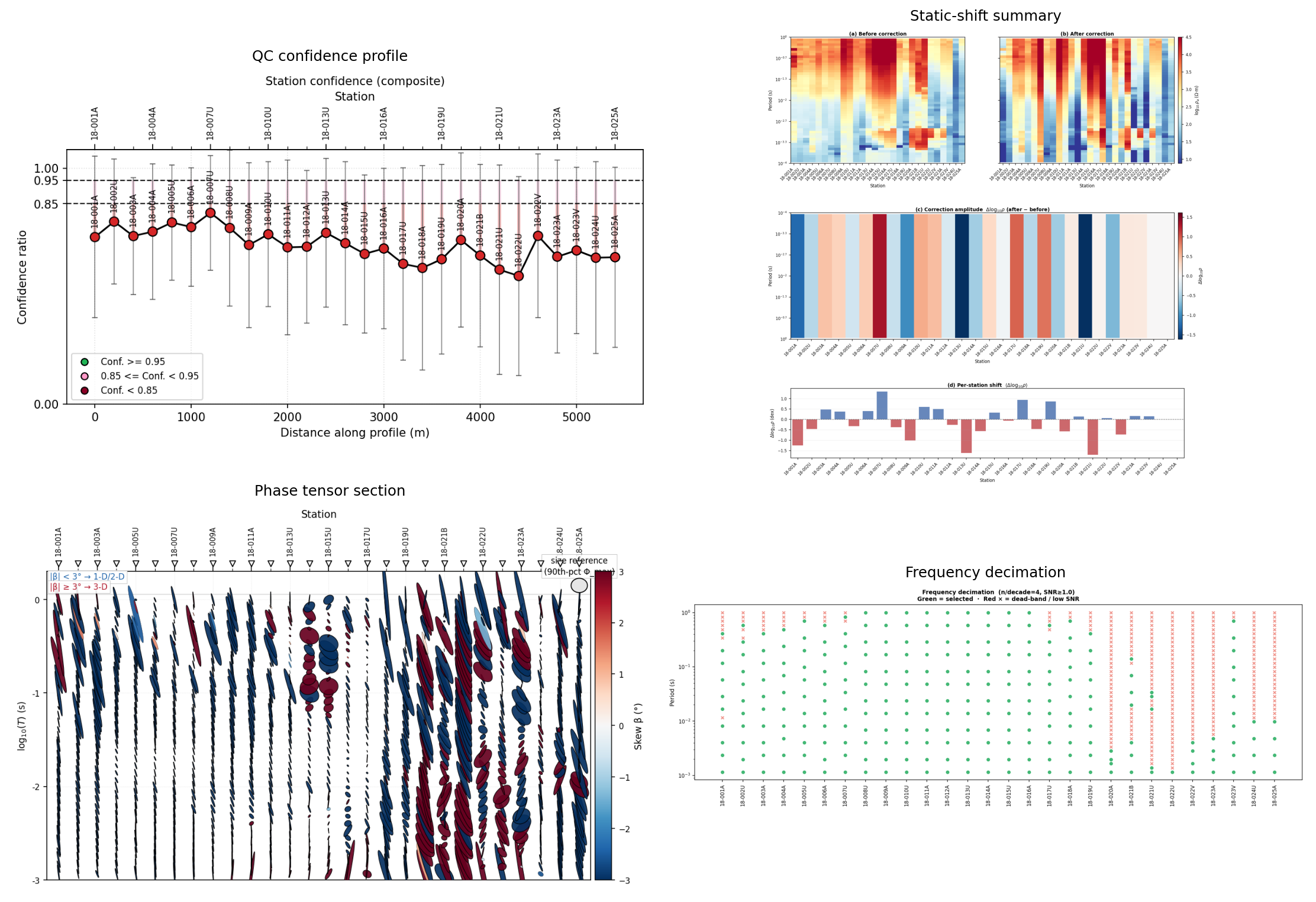
Grid of QC, static-shift, phase tensor, and frequency-decimation products for the WILLY line. — Key processing products from the WILLY L18PLT example: station confidence, static-shift correction, phase-tensor section, and period decimation. The grid lets the QC, correction, dimensionality, and period-selection decisions be reviewed together.#

Look closely at the static-shift panels and panel (b) reads as less laterally smooth than panel (a) – more station-to-station alternation, not less. That is not a mislabeled figure: \(\log_{10}\rho'_{a,i}(T) = \log_{10}\rho_{a,i}(T) - \Delta_i\) cannot change a column’s shape with period, only its level, so the identical vertical (period-to-period) roughness of the two panels is the tell that they are a genuine before/after pair rather than a swap. Measuring lateral roughness (the mean squared difference between adjacent stations at fixed period) on this line gives \(\approx 0.34\) before correction and \(\approx 1.21\) after it – correction made the section rougher, not smoother. The most defensible reading is not a bug but a mismatch between method and data: AMA correction assumes neighbouring stations share a similar true regional trend, and this line’s own phase-tensor evidence above (n_3d = 1455 against n_2d = 29 and n_1d = 0) says that assumption is a poor fit here, so a half_window=3 neighbourhood correction can end up removing some real lateral structure along with the galvanic distortion. A smooth “before” panel is not by itself evidence of a correct one; check the delta section (c) and the per-station bars (d) against independent geology or a wider half_window before trusting either panel at face value.

4.2.4. TensorRotationAgent#

TensorRotationAgent rotates impedance tensors and tipper vectors by a fixed strike angle and writes rotated EDI files. It is normally used after PhaseAnalysisAgent has estimated a stable strike, or when the analyst has a geological strike from mapping or previous modelling.

For a horizontal rotation angle \(\theta\), the impedance tensor transforms as

\[\begin{split}\mathbf{Z}' = \mathbf{R}(\theta)\, \mathbf{Z}\,\mathbf{R}^{T}(\theta), \qquad \mathbf{R}(\theta)= \begin{bmatrix} \cos\theta & \sin\theta\\ -\sin\theta & \cos\theta \end{bmatrix}.\end{split}\]

The agent audits the rotation using a diagonal-suppression proxy:

\[\Delta_{\mathrm{diag}} = \left\langle |Z_{xx}/Z_{xy}| \right\rangle_{\mathrm{before}} - \left\langle |Z'_{xx}/Z'_{xy}| \right\rangle_{\mathrm{after}}.\]

A positive value means the rotation reduced diagonal energy relative to the off-diagonal mode, which is often desirable for approximately 2-D responses. A negative or unstable value suggests the selected angle may not represent the data well.

>>> from pycsamt.agents import TensorRotationAgent
>>> rotated = TensorRotationAgent(strike_deg=-38.5).execute({
...     "path": "data/AMT/WILLY_DATA/L18PLT",
...     "output_dir": "outputs/willy_processing/rotated_edis",
...     "overwrite": True,
... })
>>> print(rotated["strike_deg"])
-38.5
>>> print(rotated["n_written"])
28
>>> print(rotated["z_diag_reduction"])
0.0654

The essential outputs are written_paths, failed_stations, n_written, z_diag_reduction, and figure_paths. Use written_paths as the hand-off to external inversion software or to EDIExportAgent-style delivery workflows.

4.2.5. TipperAnalysisAgent#

TipperAnalysisAgent analyzes vertical magnetic transfer functions when tipper data are present. Tipper vectors complement impedance diagnostics because they are sensitive to lateral conductivity gradients and 3-D structure. The agent produces a tipper table over station and period, an induction-arrow table at a reference period, and figures for amplitude, arrows, and pseudosections.

If \(T_x\) and \(T_y\) are the complex tipper components, the vertical field relation is

\[H_z = T_x H_x + T_y H_y.\]

The induction-arrow components are derived from the real or imaginary tipper parts depending on the requested convention. convention="wiese" and "parkinson" differ in arrow orientation, so keep the convention explicit in reports.

>>> from pycsamt.agents import TipperAnalysisAgent
>>> tipper = TipperAnalysisAgent(convention="wiese").execute({
...     "path": "data/AMT/WILLY_DATA/L18PLT",
...     "output_dir": "outputs/willy_processing/tipper",
... })
>>> print(tipper.status)
failed
>>> print(tipper.error)
No tipper data found in any station.

This failure is informative rather than exceptional: many AMT/CSAMT EDI collections contain impedance but no tipper section. Run this agent only when the acquisition includes vertical magnetic data.

4.2.6. FrequencyDecimationAgent#

FrequencyDecimationAgent selects a compact period set for inversion and publication plots. It removes periods outside a requested range, rejects periods that fail an SNR threshold, and keeps a log-spaced subset controlled by n_per_decade. This is especially useful before Occam2D, ModEM, AI inversion, or comparison plots where too many adjacent frequencies can overweight a narrow part of the spectrum.

Let \(T_j = 1/f_j\) be the period associated with frequency \(f_j\). After the period-range and SNR masks are applied, selected target periods are placed uniformly in \(\log_{10}T\):

\[\tau_m = \tau_{\min} + m\, \frac{\tau_{\max}-\tau_{\min}}{M-1}, \qquad \tau=\log_{10}T.\]

For each target \(\tau_m\), the nearest valid observed period is retained. The result preserves logarithmic depth coverage while avoiding unnecessary frequency density.

>>> from pycsamt.agents import DataQCAgent, FrequencyDecimationAgent
>>> qc = DataQCAgent().execute({"path": "data/AMT/WILLY_DATA/L18PLT"})
>>> decimated = FrequencyDecimationAgent(
...     n_per_decade=4,
...     snr_threshold=1.0,
... ).execute({
...     "sites": qc["sites"],
...     "period_range": [0.001, 10.0],
...     "output_dir": "outputs/willy_processing/decimated",
... })
>>> print(decimated.status)
success
>>> print(decimated["n_selected"], decimated["n_original"])
258 1092
>>> print(round(decimated["selection_ratio"], 3))
0.236

Use selected_periods when preparing inversion inputs. Use dead_band_mask to understand which stations and periods were rejected by the SNR criterion.

4.2.7. DenoisingAgent#

DenoisingAgent suppresses unstable impedance responses before analysis or inversion. Supported modes include "rpca", "hampel", "emap", "pipeline", and AI denoisers when the optional neural backend is available. The agent reports a simple SNR-proxy improvement, the number of cells that crossed the SNR threshold, and a before/after pseudosection figure.

For the RPCA mode, the conceptual model is

\[\mathbf{X} = \mathbf{L} + \mathbf{S} + \mathbf{E},\]

where \(\mathbf{X}\) is the observed response matrix, \(\mathbf{L}\) is a low-rank coherent signal, \(\mathbf{S}\) is sparse contamination, and \(\mathbf{E}\) is residual noise. The goal is not to make the data smooth; it is to preserve coherent electromagnetic structure while reducing isolated outliers and unstable bands.

>>> from pycsamt.agents import DataQCAgent, DenoisingAgent
>>> qc = DataQCAgent().execute({"path": "data/AMT/WILLY_DATA/L18PLT"})
>>> denoised = DenoisingAgent(method="rpca").execute({
...     "sites": qc["sites"],
...     "output_dir": "outputs/willy_processing/denoised",
... })
>>> print(denoised.status)
success
>>> print(round(denoised["snr_gain"], 3))
0.06
>>> print(denoised["n_recovered"])
19

Use denoised_sites as the input to AI inversion or robust downstream analysis. Keep snr_gain in context: a small positive gain may still be valuable if it recovers critical periods, while a large gain should be checked against the before/after figure to avoid over-smoothing.

4.2.8. Putting The Agents Together#

The safest production pattern is to preserve each processing state explicitly:

raw sites
-> qc["sites"]
-> shifted["corrected_sites"]
-> phase diagnostics and strike estimate
-> decimated["selected_periods"]
-> denoised["denoised_sites"] when required
-> rotated EDI files when a fixed strike frame is justified

For reproducibility, keep the output directory stable and inspect warnings after every agent. A successful status means the agent produced a usable result; it does not mean that every station, period, correction, or geological assumption is scientifically resolved.