1.8. Section Plot Layout

pycsamt.api.section is the shared layout system behind every 2-D station-by-depth or station-by-period plot pyCSAMT draws: Pseudosection QC panels, inversion sections, and compact dashboard tiles alike. It answers three questions the same way for all of them – how big should the figure be, how should the axes behave, and how should the colourbar look – through PYCSAMT_SECTION, one singleton following the same pattern as Plot Styles and Interpretation Plot Styles.

Every demonstration below uses the same real WILLY AMT line as Plot Styles:

>>> from pathlib import Path
>>> from pycsamt.emtools import ensure_sites
>>> from pycsamt.emtools.qc import plot_frequency_confidence_psection
>>> from pycsamt.api.section import PYCSAMT_SECTION

>>> edi_dir = Path("data/AMT/WILLY_DATA/L18PLT")
>>> sites = ensure_sites(
...     edi_dir,
...     recursive=True,
...     on_dup="replace",
...     strict=False,
...     verbose=0,
... )
>>> len(sites)
28

The full science behind the confidence metric itself – plot_frequency_confidence_psection()’s method/metric arguments and what “confidence” means – is covered in Quality-Control Confidence Scoring; this page only uses it as a real, data-driven anchor for the layout system.

Six presets ship with the package – "pseudosection" (the default), "inversion", "publication", "compact", "dashboard", and "dynamic" – each bundling three leaf dataclasses: SectionFigureStyle (size and margins), SectionAxisStyle (labels, y-axis direction, aspect, and what the y-axis physically represents), and SectionColorbarStyle (placement and tick density). Printing the singleton summarises all six at once:

>>> print(PYCSAMT_SECTION)
PyCSAMTSection
  compact: figsize=(7.0, 3.1), y='down', stations='pseudosection', cbar_ticks<=4
  dashboard: figsize=(6.0, 3.0), y='down', stations='pseudosection', cbar_ticks<=4
  dynamic: figsize='dynamic', y='down', stations='pseudosection', cbar_ticks<=6
  inversion: figsize=(10.5, 5.2), y='down', stations='inversion', cbar_ticks<=6
  pseudosection: figsize=(9.5, 4.4), y='down', stations='pseudosection', cbar_ticks<=6
  publication: figsize=(8.2, 3.6), y='down', stations='pseudosection', cbar_ticks<=5

1.8.1. Figure Sizing: Static Vs. Dynamic

Every preset except "dynamic" uses a fixed figsize regardless of how much data is plotted – appropriate for a consistent grid of comparison figures, but a 200-station line and a 6-station line get the same width:

>>> pub = PYCSAMT_SECTION.style_for("publication")
>>> pub.figure.figsize
(8.2, 3.6)
>>> pub.figsize_for(n_stations=6, n_y=20)
(8.2, 3.6)
>>> pub.figsize_for(n_stations=120, n_y=20)
(8.2, 3.6)

"dynamic" instead computes a width and height from the actual station count, period/depth sample count, and longest station label, then clamps the result between min_width/max_width and min_height/max_height:

>>> dyn = PYCSAMT_SECTION.style_for("dynamic")
>>> tuple(round(v, 2) for v in dyn.figsize_for(n_stations=6, n_y=20))
(7.5, 3.4)
>>> tuple(round(v, 2) for v in dyn.figsize_for(n_stations=28, n_y=40))
(7.5, 3.48)
>>> tuple(round(v, 2) for v in dyn.figsize_for(n_stations=200, n_y=40))
(15.0, 3.48)

The 200-station call hits max_width=15.0 and stops growing – a deliberate ceiling so a very long line still produces a figure that fits on a page or slide rather than growing without bound. figsize_for() is what every section-plotting function calls internally when figsize=None (the default); passing an explicit figsize= to any of them always wins over both the fixed and the dynamic calculation.

1.8.2. Named Presets In Practice

>>> for preset in ["dynamic", "publication", "compact"]:
...     ax = plot_frequency_confidence_psection(sites, section=preset, verbose=0)

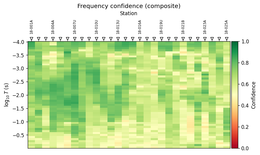
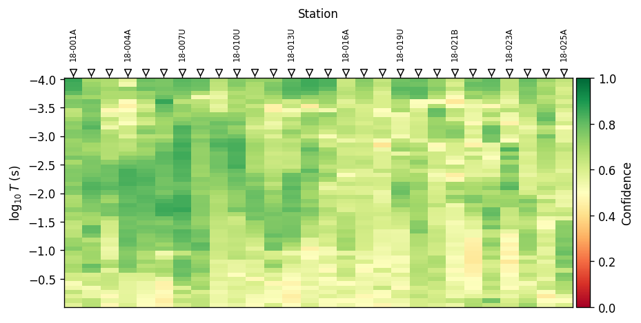
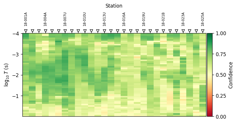
"dynamic" widens slightly for 28 real stations and keeps its own figure title; "publication" and "compact" both suppress the title (SectionAxisStyle(title=False)) and shrink progressively, trading station-label legibility for a smaller footprint – exactly the tradeoff to make deliberately rather than by trimming a figure after the fact.

1.8.3. Axis Direction And Topography Awareness

SectionAxisStyle carries a y_type tag – "period"/"frequency" for pseudosections, "depth"/"elevation" for inversion sections – that topo_active() checks against the package-wide PYCSAMT_TOPO setting. A period pseudosection carries no real elevation information, so Topography rendering is silently skipped there even when it is globally enabled – only depth-like sections pick it up:

>>> from pycsamt.topo.config import PYCSAMT_TOPO

>>> pseudo = PYCSAMT_SECTION.style_for("pseudosection")
>>> inv = PYCSAMT_SECTION.style_for("inversion")
>>> pseudo.axis.y_type, inv.axis.y_type
('period', 'depth')
>>> pseudo.topo_active(), inv.topo_active()
(False, False)

>>> _ = PYCSAMT_TOPO.configure(enabled=True)
>>> pseudo.topo_active(), inv.topo_active()
(False, True)

>>> PYCSAMT_TOPO.reset()

y_direction="down" (the default on every preset) inverts the y-axis so shallow/high-frequency values plot at the top, matching how a geologist reads a cross-section; set it to "up" or "normal" only for non-depth y-axes where that convention would be misleading.

1.8.4. Colorbar Controls

SectionColorbarStyle controls placement, width, and – most often tuned – tick density via max_ticks. Fewer ticks read better on a small multi-panel figure than the default:

>>> from pycsamt.api.section import configure_section, reset_section

>>> pub.colorbar.max_ticks
5
>>> configure_section(publication__colorbar__max_ticks=3)
>>> PYCSAMT_SECTION.publication.colorbar.max_ticks
3

>>> ax = plot_frequency_confidence_psection(sites, section="publication", verbose=0)

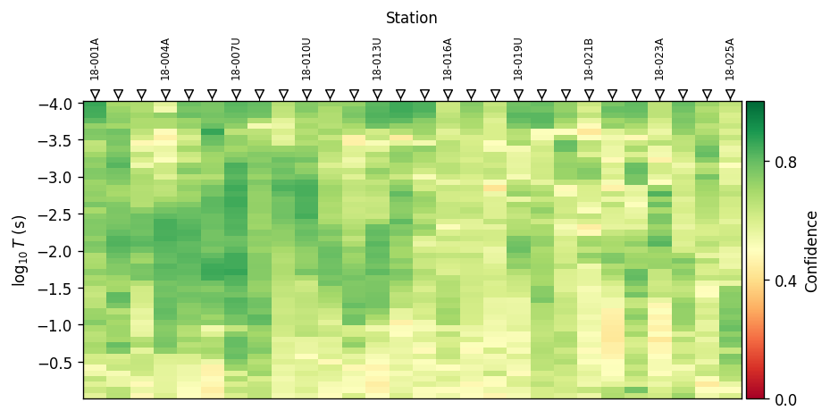
Same data and preset as the publication panel above, after lowering max_ticks to 3 – fewer labels, same underlying colour scale.

>>> reset_section()
>>> PYCSAMT_SECTION.publication.colorbar.max_ticks
5

1.8.5. Configuring And Sharing Styles

The same dotted-path configure_section() and PYCSAMT_SECTION.context() entry points used above apply to every field on every preset – figure, axis, or colorbar – and the context manager restores all six presets exactly as they were, even if the block raises:

>>> PYCSAMT_SECTION.pseudosection.figure.figsize
(9.5, 4.4)

>>> with PYCSAMT_SECTION.context("compact", pseudosection__axis__grid=True):
...     PYCSAMT_SECTION.pseudosection.figure.figsize, PYCSAMT_SECTION.pseudosection.axis.grid
((7.0, 3.1), True)

>>> PYCSAMT_SECTION.pseudosection.figure.figsize, PYCSAMT_SECTION.pseudosection.axis.grid
((9.5, 4.4), False)

PYCSAMT_SECTION.context(preset, ...) copies preset into the pseudosection slot for the duration of the block (mirroring use_preset()), applies any dotted-path overrides on top, then restores every preset – not only pseudosection – to its prior state on exit.

Each SectionStyle also carries a station_preset field ("pseudosection" or "inversion" by default) that apply_stations() uses to pull the matching station-marker style from pycsamt.api.station – station ticks, markers, and label rotation are configured separately from everything on this page, but every section preset already points at a sensible default for its own use case.

1.8.6. Next Steps

• API configuration for how the section family fits alongside every other pycsamt.api configuration family.

• Quality-Control Confidence Scoring for the frequency-confidence metric used as this page’s data anchor, and the rest of the QC pseudosection family.

• Plot Styles and Interpretation Plot Styles for the other two singleton-preset-context systems that follow this same pattern.

• Mesh Display for the layout system computational and inversion mesh figures use instead of station/period pseudosections.