
1.4. Plot Styles#
pycsamt.api.style is the single visual-style layer behind every
pycsamt.emtools figure – impedance response curves, multi-station
overlays, static-shift before/after pairs, raw-data traces, phase-tensor
ellipses, and rose diagrams alike. A plot function never hard-codes a
colour: it reads from the package-level PYCSAMT_STYLE
singleton unless the caller overrides it, so changing one setting once
changes how every subsequent figure looks.
This page walks through each of the six style families the singleton
holds, the named presets that switch all of them at once, and the
dotted-path convention (shared with every other pycsamt.api family;
see API configuration) used to tune individual attributes. All figures below
come from the real WILLY AMT line (data/AMT/WILLY_DATA/L18PLT):
>>> from pathlib import Path
>>> from pycsamt.emtools import ensure_sites
>>> from pycsamt.api.style import PYCSAMT_STYLE

>>> edi_dir = Path("data/AMT/WILLY_DATA/L18PLT")
>>> sites = ensure_sites(
...     edi_dir,
...     recursive=True,
...     on_dup="replace",
...     strict=False,
...     verbose=0,
... )
>>> len(sites)
28
The singleton prints as a compact, one-attribute-per-line summary – useful both for a sanity check after configuring it and as a map of what follows on this page:
>>> print(PYCSAMT_STYLE)
PyCSAMTStyle
  rose.bar_style          = 'gradient'
  rose.cmap               = 'YlOrRd'
  rose.compass_labels     = 'NESW'
  rose.show_mean          = True
  rose.show_secondary     = True
  multiline.mode          = 'gradient'
  multiline.base_color    = 'blue'
  multiline.dark/light    = 0.85/0.25
  mt.xy  color='#1f77b4'  marker='o'
  mt.yx  color='#d62728'  marker='s'
  mt.te  color='#1f77b4'  ls='-'
  mt.tm  color='#d62728'  ls='-'
  correction.before  color='#1f77b4'  ls='--'  label='before'
  correction.after   color='#d62728'  ls='-'  label='after'
  raw  color='black'  marker='.'  ls=':'  lw=0.8
  pt_ellipse  normalise_by='cell'  scale=0.85  c_by='skew'  cmap='RdBu_r'
  pt_ellipse  edgecolor='k'  lw=0.2  alpha=0.92  mark_3d=True  skew_thresh=3.0
Six sections, one singleton: rose (RoseStyle),
multiline (MultilineStyle), mt
(MTComponentStyle), correction
(CorrectionStyle), raw
(RawDataStyle), and pt_ellipse
(PhaseTensorEllipseStyle).
1.4.1. Named Presets#
Four presets are registered out of the box: "pycsamt" (the default –
gradient rose bars, blue/red MT colours), "publication" (grayscale,
open/filled-marker contrast for print), "dark" (brighter hues for a
dark-background notebook or slide), and "modem" (the ModEM colour
convention – pure blue/red observed, green/magenta dotted predicted).
PYCSAMT_STYLE.use() (or the
module-level use_style() shortcut) swaps every
section that a preset defines in one call:
>>> from pycsamt.api.style import use_style, reset_style
>>> from pycsamt.emtools.tensor import plot_phase_tensor_rose
>>> import matplotlib.pyplot as plt

>>> fig, axes = plt.subplots(
...     1, 3, figsize=(13, 4.6), subplot_kw={"projection": "polar"}
... )
>>> for ax, preset in zip(axes, ["pycsamt", "publication", "dark"]):
...     use_style(preset)
...     _ = plot_phase_tensor_rose(
...         sites, style=PYCSAMT_STYLE.rose, ax=ax, title=preset, verbose=0
...     )
>>> reset_style()
>>> fig.tight_layout()
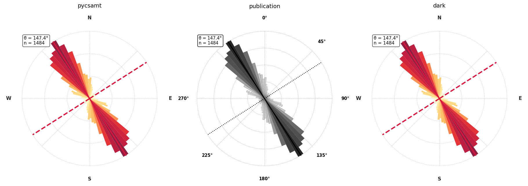
One dataset, three presets: "pycsamt" (gradient red/orange, NESW
compass), "publication" (grayscale, degree compass, dotted
conjugate line), and "dark" (same rose preset as "pycsamt" here,
since "dark" only overrides MT and multiline colours).#
"modem" is deliberately partial: its preset spec only defines an
"mt" section, so calling use_style() with it
leaves whatever rose, multiline, correction, raw, and phase-tensor
settings were already active untouched. Applying presets is therefore
compounding, not a full reset to that preset’s own defaults:
>>> reset_style()
>>> use_style("dark")
>>> PYCSAMT_STYLE.rose.cmap, PYCSAMT_STYLE.mt.xy.color
('YlOrRd', '#74b9ff')

>>> use_style("modem")
>>> PYCSAMT_STYLE.rose.cmap, PYCSAMT_STYLE.mt.xy.color
('YlOrRd', '#0000FF')
The rose colormap carries over from "dark" (which reuses the
"pycsamt" rose) because "modem" never touches it; only mt.xy
changed, to the ModEM blue. Call PYCSAMT_STYLE.reset() first if a clean, fully-defined
preset is what’s actually wanted:
>>> reset_style()
>>> PYCSAMT_STYLE.rose.cmap, PYCSAMT_STYLE.mt.xy.color
('YlOrRd', '#1f77b4')
1.4.2. MT Component Colours#
MTComponentStyle gives every impedance
component or mode (xy, yx, xx, yy, te, tm, det)
a consistent colour, marker, and line style, exposed through
plot_kwargs() and
errorbar_kwargs().
plot_response_tipper() uses it automatically
for every component it draws:
>>> from pycsamt.emtools.plot import plot_response_tipper

>>> use_style("pycsamt")
>>> fig_a = plot_response_tipper(
...     sites,
...     stations=["18-001A"],
...     components=("xy", "yx"),
...     tipper_components=(),
...     ncols_groups=1,
...     verbose=0,
... )

>>> use_style("publication")
>>> fig_b = plot_response_tipper(
...     sites,
...     stations=["18-001A"],
...     components=("xy", "yx"),
...     tipper_components=(),
...     ncols_groups=1,
...     verbose=0,
... )
>>> reset_style()
tipper_components=() is passed because L18PLT is an AMT line with no
vertical-field channel; ncols_groups=1 keeps the figure sized for a
single station instead of the function’s default three-wide grouping.
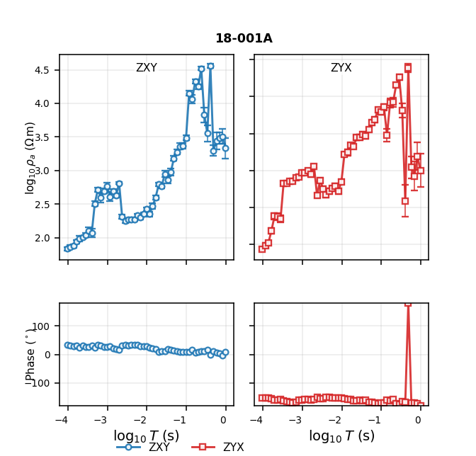
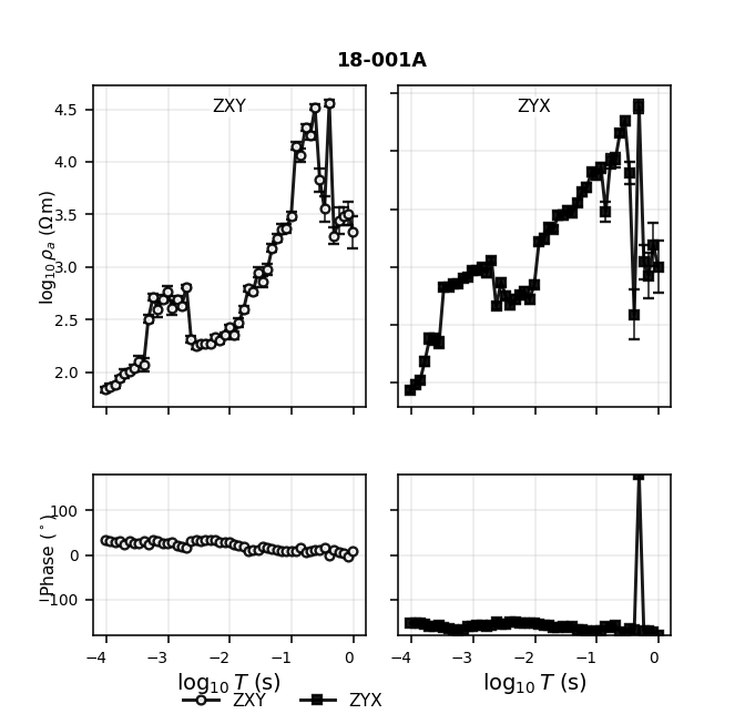
The two panels are the same station and the same data; only
PYCSAMT_STYLE.mt changed between the calls. "pycsamt" keeps the
package’s blue-XY/red-YX convention with hollow markers on both; the
grayscale "publication" preset instead distinguishes XY from YX by
marker fill (hollow circles vs. solid squares) so the two components
still read apart once colour is unavailable.
Reach for a single component’s kwargs directly when writing a custom plot function rather than calling a package one:
>>> PYCSAMT_STYLE.mt.xy.plot_kwargs()
{'color': '#1f77b4', 'ls': '-', 'lw': 1.5, 'marker': 'o', 'ms': 4.0, 'mfc': 'white', 'mew': 1.2, 'alpha': 0.9, 'label': 'XY'}
1.4.3. Multiline Gradient Colours#
MultilineStyle colours a group of related
lines – typically one per station along a profile – as shades of one
hue running from dark (line 0) to light (the last line), so the group
reads as one coherent family without needing a categorical colour cycle.
colors(n) returns the
n RGBA shades directly; line_kwargs(idx, n) is the convenience form
for a loop, combining colour with the style’s default line width and
alpha:
>>> ms = PYCSAMT_STYLE.multiline
>>> [round(float(c), 3) for c in ms.colors(4)[0]]
[0.05, 0.342, 0.631, 1.0]
>>> ms.line_kwargs(0, 4)["lw"], ms.line_kwargs(0, 4)["alpha"]
(1.5, 0.85)
Overlaying four real WILLY stations’ XY apparent resistivity shows the gradient in practice – darkest line first, lightest last, regardless of plotting order:
>>> import numpy as np

>>> stations = ["18-001A", "18-002U", "18-003A", "18-004A"]
>>> n = len(stations)
>>> fig, ax = plt.subplots(figsize=(6.4, 4.4))
>>> for idx, name in enumerate(stations):
...     st = sites[name]
...     period = 1.0 / st.freq
...     rho_xy = st.rho[:, 0, 1]
...     order = np.argsort(period)
...     _ = ax.plot(
...         period[order], rho_xy[order], **ms.line_kwargs(idx, n, label=name)
...     )
>>> _ = ax.set_xscale("log")
>>> _ = ax.set_yscale("log")
>>> _ = ax.legend(fontsize=8)
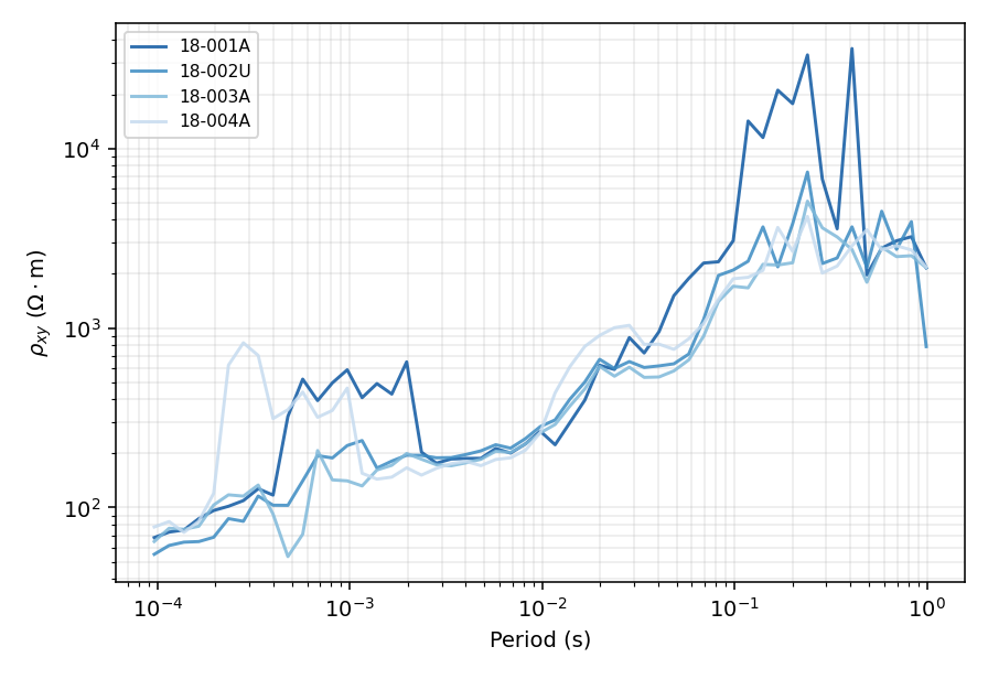
Station 18-001A (plotted first, darkest) through 18-004A
(plotted last, lightest). The gradient is keyed to plotting order,
not to any property of the data – reorder the stations list to
change which curve is darkest.#
Switch the base hue, or select an explicit colormap, with
configure():
>>> from pycsamt.api.style import configure_style
>>> configure_style(multiline__base_color="red")
>>> PYCSAMT_STYLE.multiline.cmap is None
True
>>> reset_style()
Leaving cmap unset lets base_color drive an automatic colormap
lookup ("red" -> a red sequential colormap); setting cmap
explicitly takes precedence over that lookup.
1.4.4. Before/After Correction Pairs#
Every 1-D correction workflow in pyCSAMT – static shift, near-field,
noise removal – draws its uncorrected and corrected curves with the same
CorrectionStyle pair: blue dashed for
before, red solid for after, deliberately reusing the mt.xy
and mt.yx colours so the whole package stays visually coherent.
plot_ss_station_curves() reads it directly:
>>> from pycsamt.emtools.ss import correct_ss_ama, plot_ss_station_curves

>>> corrected = correct_ss_ama(sites, verbose=0)
>>> fig, ax = plt.subplots(figsize=(6.4, 4.2))
>>> _ = plot_ss_station_curves(sites, corrected, station="18-001A", ax=ax)
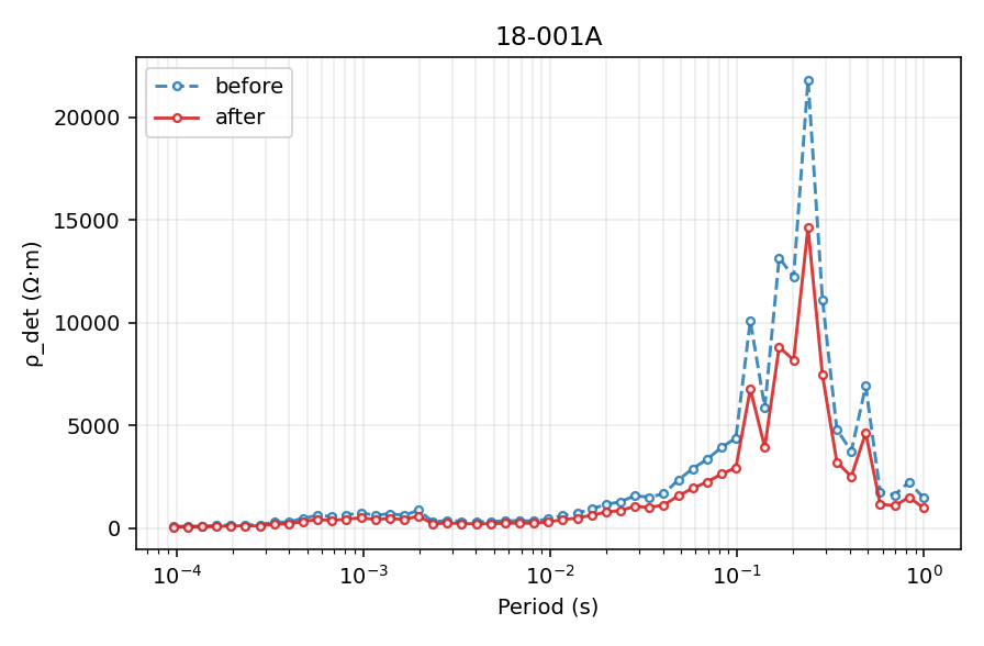
correct_ss_ama()’s real spatial-trend
correction applied to 18-001A – the AMA method estimated this
station’s determinant resistivity as offset high relative to its
neighbours and scaled it down accordingly. See Static-Shift Correction
for the correction method itself; this page is only about the pairing
convention.#
Change both curves’ colours together, or just one, with the same dotted paths used everywhere else:
>>> configure_style(
...     correction__before__color="#444444",
...     correction__after__color="#000000",
... )
>>> PYCSAMT_STYLE.correction.before.color, PYCSAMT_STYLE.correction.after.color
('#444444', '#000000')
>>> reset_style()
1.4.5. Raw Data Style#
RawDataStyle is the package’s convention for
unprocessed observations: a restrained black, thin, dotted trace with
small markers, visually distinct from any processed-data colour so a raw
curve can never be mistaken for a modelled or QC-passed one.
plot_response_tipper() switches to it
automatically whenever it is called with raw=True (unless
force_style=True asks it to keep the component colours instead):
>>> use_style("pycsamt")
>>> fig_raw = plot_response_tipper(
...     sites,
...     stations=["18-001A"],
...     components=("xy", "yx"),
...     tipper_components=(),
...     raw=True,
...     ncols_groups=1,
...     verbose=0,
... )
>>> reset_style()
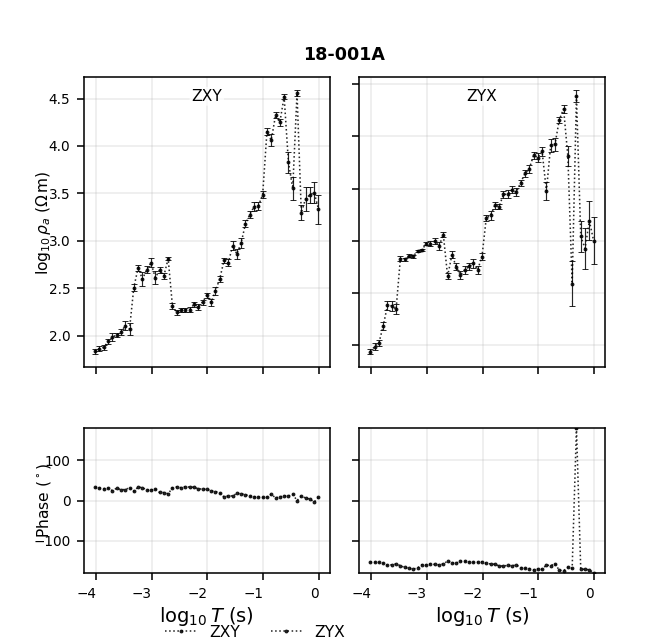
The same station and components as the MT-colours figure above,
drawn with raw=True. Colour alone now tells a reader whether a
given panel is showing raw or component-styled data, without reading
any title or legend text.#
1.4.6. Phase-Tensor Ellipse Style#
PhaseTensorEllipseStyle controls how
plot_phase_tensor_psection() and its
sibling phase-tensor figures encode five quantities at once per ellipse
– size, aspect ratio, rotation, fill colour, and a 3-D border flag. The
parameter-by-parameter tour of that encoding, including real WILLY
pseudo-sections, lives in Phase Tensor And Impedance Tensor Tools; this page
only covers the persistent-configuration angle.
c_by selects which scalar drives the fill colour, and
resolve_cmap()
looks up a sensible default colormap for it when cmap itself is left
unset – a diverging map for signed quantities like skew, a
sequential one for magnitudes like ellipticity:
>>> es = PYCSAMT_STYLE.pt_ellipse
>>> es.normalise_by, es.scale, es.c_by, es.resolve_cmap()
('cell', 0.85, 'skew', 'RdBu_r')

>>> configure_style(pt_ellipse__c_by="ellipt", pt_ellipse__cmap=None)
>>> PYCSAMT_STYLE.pt_ellipse.resolve_cmap()
'viridis'

>>> reset_style()
Any plot call can still override cmap explicitly, in which case the
c_by-based lookup above never runs – the explicit value always wins.
1.4.7. Rose Diagrams#
plot_phase_tensor_rose() and
plot_strike_rose() share
RoseStyle through their own style
keyword, which is resolved by
resolve_rose_style(). That keyword
defaults to the literal string "pycsamt" rather than to
None/the package singleton, which matters as soon as
PYCSAMT_STYLE.rose has been
configured: a bare call still resolves the named "pycsamt" preset
from resolve_rose_style’s own table, ignoring whatever the singleton
currently holds. Passing style=PYCSAMT_STYLE.rose explicitly is what
makes a rose figure track global configuration:
>>> configure_style(rose__compass_labels="degrees", rose__show_secondary=False)
>>> fig, axes = plt.subplots(
...     1, 2, figsize=(10, 4.6), subplot_kw={"projection": "polar"}
... )
>>> _ = plot_phase_tensor_rose(
...     sites,
...     style="pycsamt",
...     ax=axes[0],
...     title='style="pycsamt" (ignores singleton)',
...     verbose=0,
... )
>>> _ = plot_phase_tensor_rose(
...     sites,
...     style=PYCSAMT_STYLE.rose,
...     ax=axes[1],
...     title="style=PYCSAMT_STYLE.rose",
...     verbose=0,
... )
>>> reset_style()
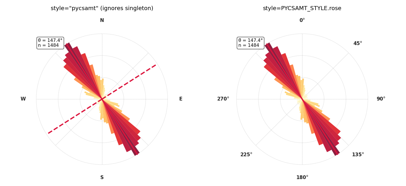
Both panels come from calls made after configure_style(rose__compass_labels="degrees",
rose__show_secondary=False). The left panel still shows a NESW
compass and the dashed conjugate line because style="pycsamt"
re-resolves the named preset from scratch; the right panel shows the
degree compass and no conjugate line, because it was handed the
singleton itself.#
The three named-preset strings ("pycsamt"/"pycsamt-rose",
"minimal", "publication") documented on
RoseStyle remain available as style=
values regardless of what PYCSAMT_STYLE.rose currently holds, since
they are resolved independently of the singleton in the same way.
1.4.8. Contour And Station-Guide Overlays#
Raster and pseudosection overlays use a separate configuration family because
they describe spatial structure rather than data-series identity. The live
pycsamt.api.PYCSAMT_CONTOUR configuration supplies contour levels,
colour, width, line style, opacity, and optional labels to compatible plots.
For example, pycsamt.emtools.plot_survey_fingerprint() uses the visible
"review" contour preset by default:
>>> from pycsamt.api import configure_contour
>>> configure_contour(linewidths=0.9, colors="#202020", alpha=0.85)
>>> fig = plot_survey_fingerprint(
...     sites,
...     render="imshow",
...     station_grid=True,
...     station_grid_kws={
...         "color": "white",
...         "linewidth": 0.65,
...         "linestyle": ":",
...         "alpha": 0.75,
...     },
... )
The contour configuration is persistent; station_grid_kws is deliberately
local to the plot call. This keeps survey-dependent station density from
silently changing unrelated figures. See Contour overlays for presets, temporary
contexts, labels, override precedence, and interpretation guidance.
1.4.9. Configuring And Sharing Styles#
Every section above is reachable through the same three entry points as
every other pycsamt.api family (see API configuration for the
general pattern): PYCSAMT_STYLE.configure() (or the module-level
configure_style()) for dotted-path edits,
direct attribute assignment for a single value, and
PYCSAMT_STYLE.context()
for a temporary change scoped to one block:
>>> PYCSAMT_STYLE.mt.xy.color
'#1f77b4'

>>> with PYCSAMT_STYLE.context("publication", mt__xy__lw=2.5):
...     PYCSAMT_STYLE.mt.xy.color, PYCSAMT_STYLE.mt.xy.lw
('black', 2.5)

>>> PYCSAMT_STYLE.mt.xy.color, PYCSAMT_STYLE.mt.xy.lw
('#1f77b4', 1.5)
The context manager restores every section (not just the ones the
preset/kw arguments touched) to exactly what it held before the
with block, even if the block raises – the same restore-on-exit
contract as PYCSAMT_MESH.context()
on Mesh Display. It is the right tool for a single figure that needs a
different look without disturbing the rest of a script or notebook
session. For a change meant to last the whole process – a batch run
producing only publication figures, for instance – call
use_style() or
configure_style() once near the top of the
script instead, and reset with reset_style()
only if a later cell or step needs package defaults back.
1.4.10. Next Steps#
API configuration for how the style family fits alongside every other
pycsamt.apiconfiguration family.Contour overlays for persistent contour presets, per-call overrides, and station-aligned vertical guides. Contours describe equal-value structure; station guides identify the shared sampling column across stacked panels.
Phase Tensor And Impedance Tensor Tools for the phase-tensor ellipse encoding itself, independent of styling.
Static-Shift Correction for the static-shift correction methods behind the before/after figure on this page.
Mesh Display for the equivalent preset system used by computational and inversion mesh figures.