1.3. Mesh Display

pycsamt.api.mesh is the shared drawing layer for every computational or inversion mesh pyCSAMT renders – resistivity sections, AI-inversion priors, solver meshes, and triangular MARE2DEM/in-house-FEM geometry alike. It centralizes how a mesh looks so that switching between mesh families or between quick-look and QC figures never means switching drawing code.

Two mesh families share one preset system:

• a structured (rectilinear) tensor grid – MaxwellMesh or GeologyGrid – drawn by draw_mesh() from 1-D cell-boundary arrays;

• an unstructured triangular mesh – TriMesh – drawn by draw_tri_mesh() from its node/triangle connectivity.

Both follow the same configure_*/reset_*/PYCSAMT_<FAMILY> pattern every other pycsamt.api family uses – see API configuration if that convention is new to you.

>>> from pycsamt.api import PYCSAMT_MESH
>>> print(PYCSAMT_MESH)
PyCSAMTMesh
  diagram: fill=False, edge=True, edge_alpha=0.9
  filled: fill=True, edge=False, edge_alpha=0.6
  review: fill=True, edge=True, edge_alpha=0.55

1.3.1. Three Presets, Shared By Both Families

Preset	Layers	Use it for
"filled" (default)	color fill only	the historical look – identical to a bare pcolormesh/ tripcolor call. Publication figures, quick looks.
"review"	color fill + cell edges	quality control: seeing exactly where cell boundaries fall relative to a resistivity anomaly, a receiver, or a topography break.
"diagram"	cell edges only, no fill	inspecting a solver mesh’s discretization before running an inversion – resolution near receivers, padding extent, triangle shape quality.

1.3.2. Structured (Rectilinear) Meshes

draw_mesh() takes 1-D, strictly monotonic cell-boundary arrays – not centres. Build them directly, or convert from a mesh contract object with edges_from_maxwell_mesh() (for a MaxwellMesh, which already stores edges) or edges_from_geology_grid() (for a GeologyGrid, which stores centres and needs cell_edges_from_centres() under the hood):

>>> import numpy as np
>>> from pycsamt.forward.maxwell import MaxwellMesh
>>> from pycsamt.api import draw_mesh, edges_from_maxwell_mesh

>>> x_edges = np.linspace(0.0, 1000.0, 11)
>>> z_edges = np.linspace(0.0, 500.0, 6)
>>> mesh = MaxwellMesh(x_edges, z_edges)
>>> mesh.shape
(5, 10)

>>> resistivity = np.full(mesh.shape, 100.0)
>>> resistivity[1:3, 3:6] = 10.0  # a shallow conductive block

>>> x_e2, z_e2 = edges_from_maxwell_mesh(mesh)
>>> np.array_equal(x_e2, x_edges), np.array_equal(z_e2, z_edges)
(True, True)

Draw the plain, filled default – no preset needed:

>>> import matplotlib.pyplot as plt
>>> fig, ax = plt.subplots(figsize=(6, 3))
>>> fill, edges = draw_mesh(ax, x_edges, z_edges, resistivity, cmap="turbo_r")
>>> fill is not None, edges is None
(True, True)

Add a colorbar the same way any pyCSAMT figure does:

>>> from pycsamt.api.plot import add_colorbar
>>> cbar = add_colorbar(fill, ax=ax, label="Resistivity (Ohm.m)")
>>> type(cbar).__name__
'Colorbar'

Switch to "review" to see the mesh boundaries drawn on top of the same fill – useful right after building a solver mesh, to confirm the anomaly sits inside the cells you expect it to:

>>> fig, ax = plt.subplots(figsize=(6, 3))
>>> fill, edges = draw_mesh(
...     ax, x_edges, z_edges, resistivity, preset="review", cmap="turbo_r"
... )
>>> fill is not None, edges is not None
(True, True)

Or drop the fill entirely with "diagram" to inspect discretization alone – values is not required (and is ignored if passed) when the fill layer is off:

>>> fig, ax = plt.subplots(figsize=(6, 3))
>>> fill, edges = draw_mesh(ax, x_edges, z_edges, preset="diagram")
>>> fill is None, edges is not None
(True, True)

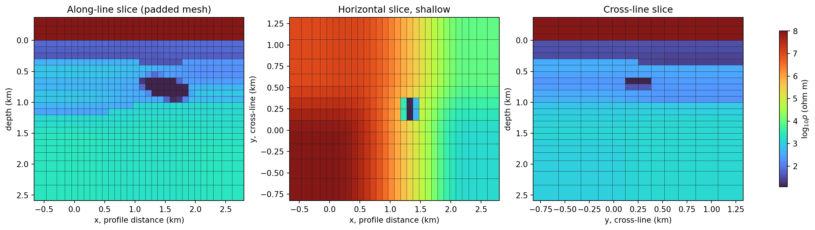
draw_mesh(..., preset="review") in real use: mesh cell boundaries drawn over a 3-D geological prior and padded solver mesh, from the porphyry-mineralization tutorial. The same overlay works whether the mesh underneath is a training prior or a converged inversion result – draw_mesh only cares about edges and cell values, not what produced them.

1.3.3. Triangular Meshes

draw_tri_mesh() is the unstructured counterpart, sharing the exact same preset objects so "filled"/"review"/"diagram" behave identically. It takes per-triangle values (not per-node) and builds a matplotlib.tri.Triangulation internally via triangulation_from_tri_mesh():

>>> from scipy.spatial import Delaunay
>>> from pycsamt.forward.maxwell import TriMesh
>>> from pycsamt.api import draw_tri_mesh

>>> xs = np.linspace(0.0, 1000.0, 6)
>>> zs = np.linspace(0.0, 500.0, 4)
>>> xx, zz = np.meshgrid(xs, zs)
>>> points = np.column_stack([xx.ravel(), zz.ravel()])
>>> tri = Delaunay(points)
>>> tri_mesh = TriMesh(points, tri.simplices, boundary_segments=tri.convex_hull)
>>> tri_mesh.n_nodes, tri_mesh.n_triangles
(24, 30)

>>> tri_values = np.full(tri_mesh.n_triangles, 100.0)
>>> cx = tri_mesh.triangle_centroids_m[:, 0]
>>> cz = tri_mesh.triangle_centroids_m[:, 1]
>>> tri_values[(cx > 300) & (cx < 700) & (cz < 250)] = 10.0  # same block

>>> fig, ax = plt.subplots(figsize=(6, 3))
>>> fill, edges = draw_tri_mesh(
...     ax, tri_mesh, tri_values, preset="review", cmap="turbo_r"
... )
>>> fill is not None, edges is not None
(True, True)
>>> ax.invert_yaxis()  # depth positive down, matching the rectilinear path

A TriMesh built by build_survey_mesh() already has its node z-coordinates following real topography – the mesh’s own top boundary is the topo line. Unlike the rectilinear build_topo_section() path, which warps a flat regular grid onto a terrain surface by interpolation, draw_tri_mesh needs no separate drape step: plotting the mesh’s own coordinates on a depth-positive-down axis already shows a topography-draped section.

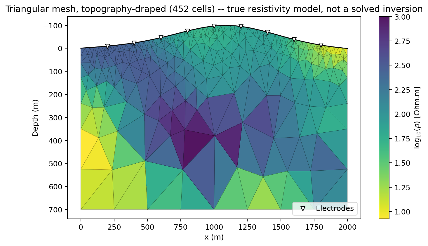
draw_tri_mesh with a real topography-following triangulation, a correlated resistivity field, and electrode markers (from StationMarkerStyle()) – the filled section look every triangular-mesh AI-inversion figure in the ai_inversion guide shares.

That true-model figure only paints the target field; the same call renders a genuinely solved AI inversion just as directly, since draw_tri_mesh never distinguishes “true” from “predicted” – both are just a per-triangle array:

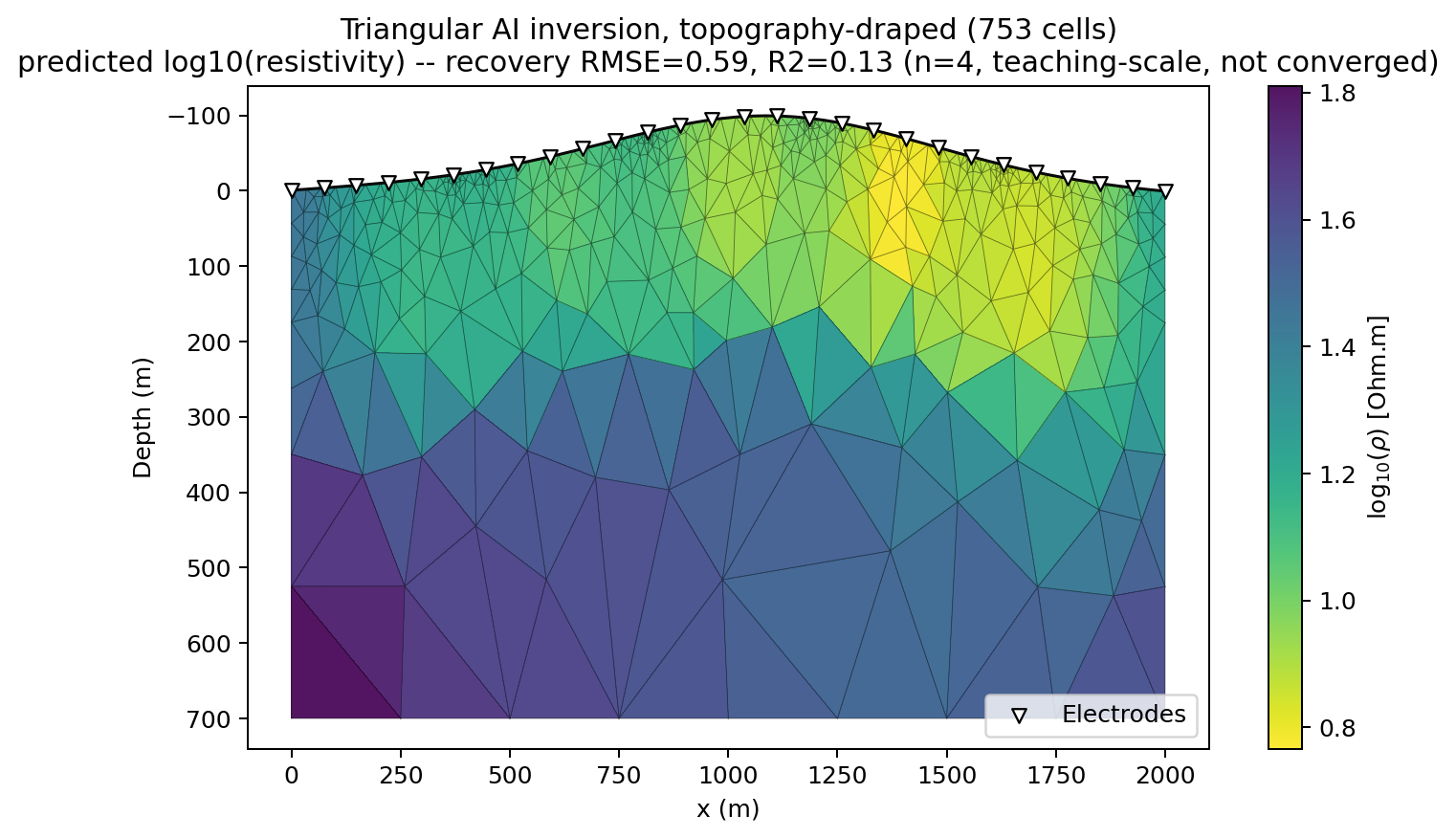
A genuine Inv2DAgent(physics="mt2d_tri", topo_x_m=..., topo_z_m=...) run – real WILLY station geometry, synthetic training topography and geology, teaching-scale (not converged, recovery metrics reported plainly in the title) – on the same topography-draped mesh style. Receivers sitting on real, non-flat terrain needed a real fix first, not just a mesh change: see TriFEM2DAdapter’s own module docstring for the surface-detection generalization this required.

1.3.4. Configuring Mesh Styles

Every mesh-display attribute follows the same dotted-path convention as every other pycsamt.api family (see Configuration): preset__layer__attribute.

>>> from pycsamt.api import configure_mesh, reset_mesh

>>> configure_mesh(review__edge__alpha=0.4, review__edge__linewidth=0.25)
>>> PYCSAMT_MESH.style_for("review").edge.alpha
0.4
>>> PYCSAMT_MESH.style_for("review").edge.linewidth
0.25

>>> reset_mesh()
>>> PYCSAMT_MESH.style_for("review").edge.alpha
0.55

Use PYCSAMT_MESH.context() when only one figure needs a different style – the previous configuration is restored afterward even if the block raises:

>>> with PYCSAMT_MESH.context(review__edge__alpha=0.3):
...     PYCSAMT_MESH.style_for("review").edge.alpha
0.3
>>> PYCSAMT_MESH.style_for("review").edge.alpha
0.55

An explicit MeshStyle passed as style= always overrides preset for a single call, without touching global configuration at all:

>>> from pycsamt.api import MeshStyle, MeshEdgeStyle
>>> custom = MeshStyle(edge=MeshEdgeStyle(show=True, color="white", linewidth=0.2))
>>> fig, ax = plt.subplots(figsize=(6, 3))
>>> fill, edges = draw_mesh(ax, x_edges, z_edges, resistivity, style=custom)
>>> fill is not None, edges is not None
(True, True)

1.3.5. Next Steps

• API configuration for how the mesh family fits alongside every other pycsamt.api configuration family.

• Configuration for the dotted-path convention shared by all families, and recommended session setups.

• Architecture roadmap for where meshes come from in an AI-inversion workflow – MaxwellMesh and TriMesh are both solver-neutral contracts built well before any figure is drawn.

• MARE2DEM for build_survey_mesh(), the real topography-following triangulation behind the gallery figure above.

• pycsamt.api for the full generated reference, including every MeshStyle field.