
1.9. Station Rendering#
pycsamt.api.station draws the station axis on every 2-D section
figure: the tick marks, thinned labels, and marker glyphs along the
profile edge. Section Plot Layout already introduced how
apply_stations() looks up a
station style by name through this module’s own singleton,
PYCSAMT_STATION_RENDERING; this page covers
that singleton directly – its three presets, the adaptive label-thinning
algorithm, and the terrain-following marker mode.
>>> from pathlib import Path
>>> import numpy as np
>>> from pycsamt.emtools import ensure_sites
>>> from pycsamt.api.station import PYCSAMT_STATION_RENDERING

>>> edi_dir = Path("data/AMT/WILLY_DATA/L18PLT")
>>> sites = ensure_sites(
...     edi_dir,
...     recursive=True,
...     on_dup="replace",
...     strict=False,
...     verbose=0,
... )
>>> names = [s.name for s in sites]
>>> x = np.arange(len(names)) * 200.0
>>> len(names)
28
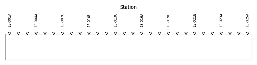
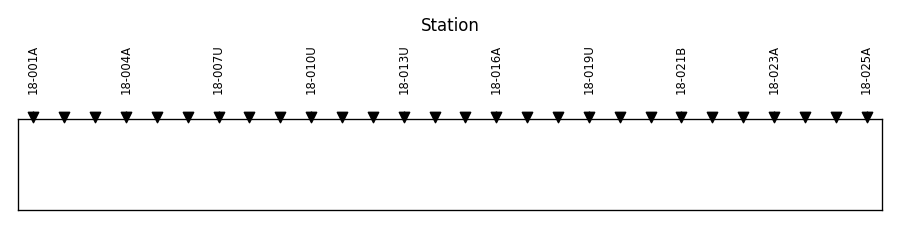
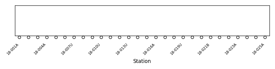
Three presets ship with the package – "pseudosection" (hollow white
triangles, top axis), "inversion" (filled black triangles, top axis),
and "survey" (hollow white circles, bottom axis, diagonal labels).
Each pairs a StationAxisStyle (ticks,
labels, side) with its own StationMarkerStyle
(glyph, size, colours):
>>> print(PYCSAMT_STATION_RENDERING)
PyCSAMTStationRendering
  pseudosection: side='top', marker='v', face='white', labels<=14
  inversion: side='top', marker='v', face='black', labels<=14
  survey: side='bottom', marker='o', face='white', labels<=14
apply() draws directly
onto any axes given station positions and labels – no section plot
required:
>>> import matplotlib.pyplot as plt
>>> for preset in ["pseudosection", "inversion", "survey"]:
...     fig, ax = plt.subplots(figsize=(7.5, 1.9))
...     _ = ax.set_xlim(x.min() - 100, x.max() + 100)
...     _ = ax.set_ylim(0, 1)
...     _ = ax.set_yticks([])
...     idx = PYCSAMT_STATION_RENDERING.apply(ax, x, names, preset=preset)
1.9.1. Adaptive Label Thinning#
Only 28 stations fit their names comfortably in a 7.5-inch figure – every
third label above – but compute_every()
scales the same decision to any station count and figure width, always
returning a “nice” step (1, 2, 3, 4, 5, 8, 10, 12, 15, 20, 25, 50, 100, …)
rather than an arbitrary number:
>>> pseudo = PYCSAMT_STATION_RENDERING.style_for("pseudosection")
>>> pseudo.compute_every(28)
2
>>> pseudo.compute_every(100)
8
>>> pseudo.compute_every(500)
50
>>> pseudo.compute_every(500, figwidth_in=15)
25
A wider figure earns a smaller step – 500 stations at the default
10-inch reference width thin to every 50th label, but the same 500
stations on a 15-inch figure fit every 25th. every defaults to
"auto" (this algorithm); set it to a fixed integer on any preset to
bypass the computation entirely, e.g.
configure_station_rendering(pseudosection__every=5).
label_indices() runs the same
computation and returns the actual visible indices, always including the
last station regardless of step, which is why the demo above ends on
index 27 rather than stopping wherever the step last landed.
Note that compute_every alone uses whatever figwidth_in is passed
to it (10.0 by default), while apply()
– what every real plot call goes through – reads the actual figure’s
width automatically, which is why the three-preset figures above (7.5
inches wide) thinned to every third label rather than every second.
1.9.2. Topography-Aware Marker Placement#
By default, station markers sit at a flat position along the axis edge
regardless of what the section shows underneath – appropriate for
Pseudosection panels, which have no real elevation information
either (see Section Plot Layout’s topography-awareness gate). Pass
topo_elev= to apply() and
markers instead ride the real terrain surface, with labels drawn inline
above each one instead of as axis tick labels:
>>> elev = 1200.0 + 40.0 * np.sin(np.linspace(0, 3.0, len(names)))
>>> fig, axes = plt.subplots(1, 2, figsize=(11, 3.2))

>>> ax0 = axes[0]
>>> _ = ax0.plot(x, elev, color="0.5", lw=1)
>>> _ = ax0.set_ylim(elev.min() - 60, elev.max() + 60)
>>> _ = pseudo.apply(ax0, x, names, xlim=(x.min() - 100, x.max() + 100))
>>> _ = ax0.set_title("flat-datum mode (default)")

>>> ax1 = axes[1]
>>> _ = ax1.plot(x, elev, color="0.5", lw=1)
>>> _ = ax1.set_ylim(elev.min() - 60, elev.max() + 60)
>>> _ = pseudo.apply(
...     ax1, x, names, xlim=(x.min() - 100, x.max() + 100), topo_elev=elev,
... )
>>> _ = ax1.set_title("topo_elev= mode")
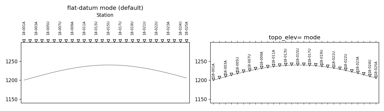
elev here is an illustrative sine curve, not real WILLY terrain –
the point is the mechanic, not the geology. In practice topo_elev
comes from PYCSAMT_TOPO’s elevation
source once topo_active()
is True for a depth-like section; Section Plot Layout covers that gate.#
1.9.3. Configuring And Sharing Styles#
The same dotted-path configure_station_rendering()
and PYCSAMT_STATION_RENDERING.context()
entry points from every other pycsamt.api family apply here too.
The context manager copies a named preset into the pseudosection slot
for the block (mirroring
use_preset()) and
restores all three presets afterward:
>>> from pycsamt.api.station import configure_station_rendering, reset_station_rendering

>>> PYCSAMT_STATION_RENDERING.pseudosection.side, PYCSAMT_STATION_RENDERING.pseudosection.marker.marker
('top', 'v')

>>> with PYCSAMT_STATION_RENDERING.context("survey", pseudosection__rotation=30.0):
...     (
...         PYCSAMT_STATION_RENDERING.pseudosection.side,
...         PYCSAMT_STATION_RENDERING.pseudosection.marker.marker,
...         PYCSAMT_STATION_RENDERING.pseudosection.rotation,
...     )
('bottom', 'o', 30.0)

>>> (
...     PYCSAMT_STATION_RENDERING.pseudosection.side,
...     PYCSAMT_STATION_RENDERING.pseudosection.marker.marker,
...     PYCSAMT_STATION_RENDERING.pseudosection.rotation,
... )
('top', 'v', 90.0)
A dotted path descends into the nested marker dataclass the same way
it descends into any other family’s leaf styles:
>>> configure_station_rendering(
...     inversion__marker__facecolor="crimson",
...     inversion__max_labels=20,
... )
>>> PYCSAMT_STATION_RENDERING.inversion.marker.facecolor
'crimson'

>>> reset_station_rendering()
>>> PYCSAMT_STATION_RENDERING.inversion.marker.facecolor
'black'
1.9.4. Next Steps#
Section Plot Layout for how
station_preseton aSectionStyleselects one of these three presets automatically, and for the topography-awareness gate that decides whentopo_elevis actually available.API configuration for how the station-rendering family fits alongside every other
pycsamt.apiconfiguration family.Plot Styles and Interpretation Plot Styles for the other singleton-preset systems that follow the same configuration pattern.