3. CSAMT, AMT, and MT Overview#

pyCSAMT works with several related electromagnetic (EM) sounding methods: magnetotellurics (MT), audio-frequency magnetotellurics (AMT), controlled-source audio-frequency magnetotellurics (CSAMT), controlled-source EM (CSEM), and time-domain EM (TDEM). They share the same physical foundation: electrical conductivity controls how time-varying EM fields diffuse through the Earth. They differ mainly in source type, frequency band, acquisition geometry, and the assumptions that are safe during interpretation.

This page gives the conceptual background needed before reading the more specific pages on Impedance Tensor, Static Shift, and Inversion Concepts. It assumes the notation and constants introduced in Prerequisites and Physical And Geodetic Constants – \(\rho\), \(\omega\), \(\mu_0\), and the rest of the vocabulary used below are defined there, not re-derived here.

3.1. Why Resistivity Matters#

Most pyCSAMT workflows are ultimately trying to estimate subsurface resistivity, commonly denoted \(\rho\), or its inverse conductivity, \(\sigma\):

(1)#\[\rho = \frac{1}{\sigma}.\]

In geophysical EM methods, resistivity is not measured directly. The field system measures electric and magnetic fields at the surface or near the surface. Those fields are then transformed into response functions such as impedance tensor, apparent resistivity, phase, tipper, or transient decay curves. The interpreter uses those responses to infer geological structure.

Resistivity is useful because rocks, fluids, alteration zones, graphite, sulfides, clay, salinity, porosity, permeability, temperature, and fracture connectivity can all influence bulk electrical behavior. A resistivity model is therefore not a lithology map by itself; it is a physical property model that must be interpreted with geology, boreholes, geochemistry, hydrology, and survey context.

3.2. The Family Of Methods#

The methods supported by pyCSAMT can be grouped by source.

Method	Source	Typical domain	Main interpretation concern
MT	Natural ionospheric and magnetospheric variations	Broad frequency band, often deep investigation	Assumes a plane-wave field natural source at the survey scale.
AMT	Natural audio-frequency variations	Higher frequencies than long-period MT, shallower targets	Signal strength can be weak or culturally noisy in the audio band.
CSAMT	Controlled-source grounded electric dipole	Audio-frequency controlled-source sounding	Must distinguish far field behavior from near field and transition field source effects.
CSEM	Controlled electric or magnetic source	Frequency-domain controlled-source EM	Source geometry and full transmitter-receiver coupling are part of the forward problem.
TDEM	Controlled transient source	Time-domain decay after source turn-off	Interpretation depends on transient diffusion and gate timing rather than steady harmonic impedance.

Frequency-domain methods use harmonic signals with angular frequency \(\omega\):

(2)#\[\omega = 2 \pi f,\]

where \(f\) is frequency in hertz. The period is:

(3)#\[T = \frac{1}{f}.\]

High frequencies generally sample shallower structure; low frequencies sample deeper structure. This is not a hard boundary, because sensitivity also depends on resistivity, dimensionality, noise, source geometry, and the inversion model. The next two sections make that scale precise, first through Maxwell’s equations and then through skin depth.

3.3. Maxwell Equations In The Diffusive Regime#

MT, AMT, CSAMT, and many CSEM workflows operate at frequencies where subsurface EM behavior is usually described by a diffusive approximation. Starting from Maxwell equations in the frequency domain:

(4)#\[\nabla \times \mathbf{E} = - i \omega \mu \mathbf{H},\]

(5)#\[\nabla \times \mathbf{H} = \mathbf{J}_s + \sigma \mathbf{E} + i \omega \epsilon \mathbf{E},\]

where \(\mathbf{E}\) is electric field, \(\mathbf{H}\) is magnetic field, \(\mathbf{J}_s\) is a source current density, \(\sigma\) is conductivity, \(\mu\) is magnetic permeability, and \(\epsilon\) is dielectric permittivity.

For many geophysical EM surveys in conductive Earth materials, the displacement current term \(i \omega \epsilon \mathbf{E}\) in (5) is small relative to the conduction current \(\sigma \mathbf{E}\). The working equation becomes approximately:

(6)#\[\nabla \times \mathbf{H} \approx \mathbf{J}_s + \sigma \mathbf{E}.\]

“Small” can be made concrete rather than asserted: the ratio of conduction to displacement current is \(\sigma / (\omega \varepsilon) = 1 / (\rho\, \omega\, \varepsilon)\). Using pycsamt.constants.EPSILON_0 for a vacuum-like permittivity and a crustal resistivity of \(100\,\Omega\cdot\)m at the top of the AMT band:

>>> from pycsamt.constants import TAU, EPSILON_0
>>> rho, f = 100.0, 1000.0  # crustal resistivity, upper AMT band
>>> omega = TAU * f
>>> conduction_to_displacement = 1.0 / (rho * omega * EPSILON_0)
>>> round(conduction_to_displacement)
179751

Conduction current outweighs displacement current by more than five orders of magnitude even at 1 kHz, comfortably inside the AMT/CSAMT band – and the ratio only grows at the lower frequencies typical of MT, since it scales as \(1/f\). This is why EM sounding across the whole MT/AMT/CSAMT range is described as diffusion rather than wave propagation. EM energy diffuses downward and laterally, with a penetration scale controlled by resistivity and frequency rather than propagating at a fixed wave speed.

3.4. Skin Depth#

A useful first-order scale is the skin depth \(\delta\), the distance over which a plane EM field decays by a factor of \(e^{-1}\) in a uniform half-space:

(7)#\[\delta = \sqrt{\frac{2 \rho}{\omega \mu}} = \sqrt{\frac{\rho}{\pi f \mu}}.\]

Assuming non-magnetic rocks with \(\mu \approx \mu_0\), a common field approximation is:

(8)#\[\delta \approx 503 \sqrt{\frac{\rho}{f}},\]

where \(\delta\) is in metres, \(\rho\) is in ohm-m, and \(f\) is in hertz. The 503 is not an arbitrary round number – it is \(1/\sqrt{\pi\mu_0}\), the same combination of constants documented in Physical And Geodetic Constants. pyCSAMT actually carries this shortcut in more than one place, each rounded slightly differently:

>>> from pycsamt.interp.petrophysics import skin_depth
>>> from pycsamt.core.base import MTBase
>>> rho, f = 100.0, 100.0
>>> skin_depth(rho, f)
503.3
>>> float(MTBase().skin_depth(f, rho))
503.2921210448704

pycsamt.interp.petrophysics.skin_depth() rounds its constant to 503.3, pycsamt.core.base.MTBase computes the exact (7) from \(\mu_0\) directly (giving 503.2921...), and two further copies exist elsewhere in the codebase – pycsamt.iot.edge_csamt.skin_depth_m() uses 503.29, while pycsamt.map._core.skin_depth_at_frequency() rounds to a plain 503.0. All four agree to within a few parts in ten thousand, well below the uncertainty in any real resistivity estimate, so the rounding choice does not matter in practice – but it is the same local-duplicate pattern already noted for RHO_FACTOR in Physical And Geodetic Constants, not four independent derivations.

Skin depth should not be read as “the investigation depth.” It is a scale for a uniform Earth. Real sensitivity depends on the full conductivity distribution and on the measured response. Still, it gives a useful intuition, made concrete below for four representative resistivities across the MT and AMT/CSAMT bands:

import numpy as np
import matplotlib.pyplot as plt
from pycsamt.interp.petrophysics import skin_depth

freq = np.logspace(-3, 4, 300)  # 0.001 Hz - 10 kHz
rhos = [1.0, 10.0, 100.0, 1000.0]

fig, ax = plt.subplots(1, 1, figsize=(7.2, 4.4))
colors = plt.cm.viridis(np.linspace(0.15, 0.9, len(rhos)))
for rho, c in zip(rhos, colors):
    delta = skin_depth(rho, freq)
    ax.loglog(freq, delta, color=c, lw=2.0, label=fr"$\rho={rho:g}\,\Omega\cdot$m")

ax.axvspan(1.0, 1.0e4, color="#d62728", alpha=0.05)
ax.axvspan(1.0e-3, 1.0, color="#1f77b4", alpha=0.05)
ax.text(15, ax.get_ylim()[1] * 0.5, "AMT / CSAMT band", color="#d62728", fontsize=8)
ax.text(1.3e-3, ax.get_ylim()[1] * 0.5, "long-period MT", color="#1f77b4", fontsize=8)
ax.set(xlabel="Frequency (Hz)", ylabel=r"Skin depth $\delta$ (m)",
       title=r"$\delta \approx 503\sqrt{\rho/f}$ across resistivities")
ax.legend(fontsize=8)
ax.grid(True, which="both", alpha=0.3)
fig.tight_layout()

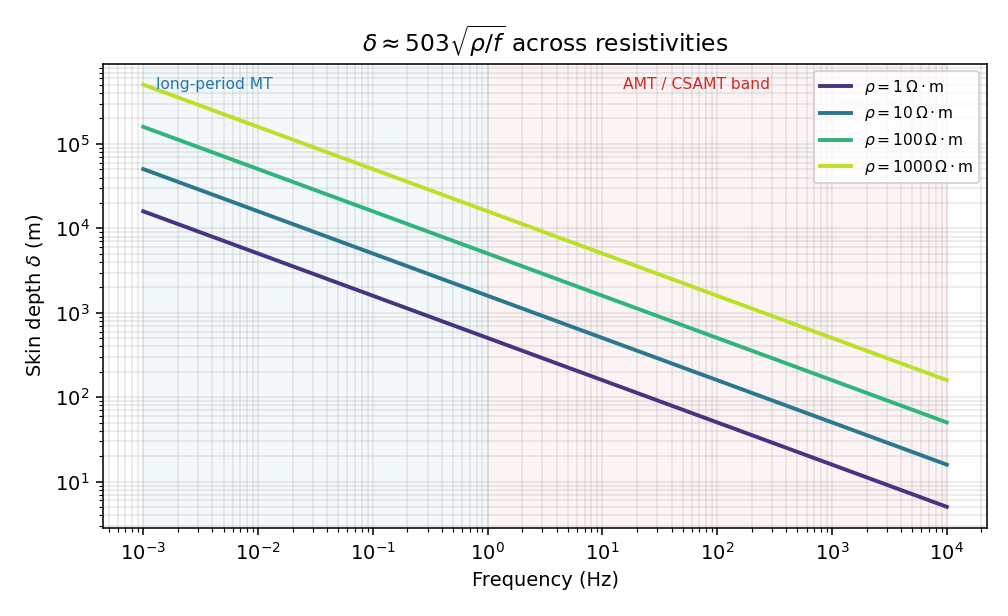
Skin depth versus frequency for four resistivities, with MT and AMT/CSAMT frequency bands shaded — Skin depth spans nearly four decades (metres to tens of kilometres) across the resistivities and frequencies a single survey might combine. A resistive \(1000\,\Omega\cdot\)m section is sampled roughly 30 times deeper than a \(1\,\Omega\cdot\)m conductor at the same frequency – the same frequency band probes very different depths depending on what is actually in the ground.#

decreasing frequency increases penetration;
increasing resistivity increases penetration;
conductive cover can strongly attenuate high-frequency fields;
shallow conductors may screen deeper targets.

3.5. MT And AMT#

MT uses naturally occurring EM fields. At suitable distances from source regions, these fields can be approximated as a plane-wave field incident on the Earth. Under the plane-wave assumption, the horizontal electric and magnetic fields at a station are related by a complex impedance tensor:

(9)#\[\begin{split}\begin{bmatrix} E_x \\ E_y \end{bmatrix} = \begin{bmatrix} Z_{xx} & Z_{xy} \\ Z_{yx} & Z_{yy} \end{bmatrix} \begin{bmatrix} H_x \\ H_y \end{bmatrix}.\end{split}\]

The tensor components vary with frequency. From them, one computes apparent resistivity and phase. A common component-wise apparent resistivity is:

(10)#\[\rho_{a,ij} = \frac{1}{\mu_0 \omega} \left| Z_{ij} \right|^2,\]

and the impedance phase is:

(11)#\[\phi_{ij} = \tan^{-1} \left( \frac{\operatorname{Im}(Z_{ij})} {\operatorname{Re}(Z_{ij})} \right).\]

Impedance Tensor derives both in full and connects them to Physical And Geodetic Constants’s RHO_FACTOR; this page only needs the shape of the relation before introducing the controlled-source complication below.

AMT is usually treated as the audio-frequency subset of MT. It is useful for shallower surveys because high frequencies have shorter skin depths. AMT surveys are often sensitive to:

near-surface conductivity variations;
cultural noise in the audio band;
weak natural-field intervals;
static shift of apparent resistivity;
station-to-station consistency and frequency coverage.

pyCSAMT processing pages and pipeline steps often use MT/AMT language even when the same operation is useful for CSAMT impedance-like data. The important question is whether the response can be treated as an impedance response under the assumptions of the workflow – which is exactly what the field-zone diagnostic below answers.

3.6. CSAMT#

CSAMT uses a controlled-source, commonly a grounded dipole transmitter, and measures fields at receivers along one or more profiles. The controlled source improves signal repeatability and can be extremely useful when natural AMT signal levels are weak or cultural noise is high.

The price is that the source is no longer “infinitely far away.” Receiver responses may contain source-field geometry, near-field effects, transition zone behavior, source overprint, and shadow effects. These issues are central to CSAMT methodology and are discussed in references such as [Yan2004], [Chen2005], [Da2016], [WangLin2023], and [Zhang2021].

For a grounded electric dipole source, the transmitter-receiver offset \(r\), transmitter length, Earth resistivity, frequency, and survey layout all affect whether a station behaves like a far-field MT-style measurement. In the far field, CSAMT responses can often be interpreted with MT-like apparent resistivity and phase concepts. In the near field or transition zone, direct MT-style interpretation can be misleading.

3.7. Field Zones In CSAMT#

CSAMT interpretation often separates measurements into approximate field zones:

Zone	Qualitative behavior	Interpretation risk
Near field	Source geometry dominates part of the measured field.	MT-like apparent resistivity may reflect source coupling rather than subsurface layering alone.
Transition field	Both source geometry and diffusive Earth response matter.	Apparent resistivity curves may show source overprint, shadow effects, or frequency-dependent distortion.
Far field	The source field approximates a plane-wave-like response at receivers.	MT-style impedance interpretation is more defensible, though noise, static shift, and dimensionality still matter.

There is no universal single number that separates these zones for all surveys. A practical diagnostic uses the ratio between transmitter-receiver offset and an EM length scale such as skin depth. Let:

(12)#\[\eta = \frac{r}{\delta}.\]

Large \(\eta\) values tend to be more far-field-like, while small \(\eta\) values tend to be more source-dominated. This is exactly what pycsamt.iot.edge_csamt.classify_field_zones() computes per frequency, using \(\eta \le 1\) as its near-field default and \(\eta \ge 3\) as its far-field default. Running it on a common CSAMT transmitter comb (powers of two from 1 Hz to 8192 Hz), a 1 km transmitter-receiver offset, and a \(100\,\Omega\cdot\)m half-space:

>>> import numpy as np
>>> from pycsamt.iot.edge_csamt import classify_field_zones
>>> freq = np.array(
...     [1, 2, 4, 8, 16, 32, 64, 128, 256, 512, 1024, 2048, 4096, 8192],
...     dtype=float,
... )
>>> coverage = classify_field_zones(freq, resistivity=100.0, offset_m=1000.0)
>>> coverage.n_near, coverage.n_transition, coverage.n_far
(5, 3, 6)
>>> round(coverage.far_fraction, 3)
0.429
>>> coverage.first_far_field_hz()
256.0
>>> coverage.correction_recommended
True
>>> coverage.zones
['near', 'near', 'near', 'near', 'near', 'transition', 'transition', 'transition', 'far', 'far', 'far', 'far', 'far', 'far']

Only 256 Hz and above reach the far field at this offset and resistivity; everything from 1 Hz to 16 Hz stays near-field, and 32-128 Hz sits in the transition zone. correction_recommended is True precisely because more than a third of the comb never reaches the far-field threshold. The same run, plotted as skin depth against the fixed 1 km offset and as the \(\eta\) ratio against its near/far thresholds, makes the crossover visible directly:

import numpy as np
import matplotlib.pyplot as plt
from pycsamt.iot.edge_csamt import classify_field_zones, skin_depth_m

freq2 = np.logspace(0, 4, 400)
offset_m = 1000.0
rho0 = 100.0
delta2 = skin_depth_m(rho0, freq2)
ratio2 = offset_m / delta2

coverage = classify_field_zones(
    np.array([1, 2, 4, 8, 16, 32, 64, 128, 256, 512, 1024, 2048, 4096, 8192],
             dtype=float),
    rho0, offset_m,
)
zone_color = {"near": "#d62728", "transition": "#ff7f0e", "far": "#2ca02c"}

fig, axes = plt.subplots(1, 2, figsize=(10.0, 4.2))
ax = axes[0]
ax.loglog(freq2, delta2, color="0.3", lw=1.8, label=r"$\delta(f)$")
ax.axhline(offset_m, color="black", lw=1.2, ls="--", label=f"offset r={offset_m:g} m")
for f, d, z in zip(coverage.freq_hz, coverage.skin_depth_m, coverage.zones):
    ax.scatter([f], [d], color=zone_color[z], zorder=5, s=28)
ax.set(xlabel="Frequency (Hz)", ylabel=r"Skin depth $\delta$ (m)",
       title=r"$\delta(f)$ vs transmitter offset")
ax.legend(fontsize=8)
ax.grid(True, which="both", alpha=0.3)

ax = axes[1]
ax.semilogx(freq2, ratio2, color="0.3", lw=1.8)
ax.axhline(1.0, color=zone_color["near"], lw=1.0, ls=":", label="near_ratio=1.0")
ax.axhline(3.0, color=zone_color["far"], lw=1.0, ls=":", label="far_ratio=3.0")
for f, r, z in zip(coverage.freq_hz, coverage.offset_ratio, coverage.zones):
    ax.scatter([f], [r], color=zone_color[z], zorder=5, s=28)
ax.set(xlabel="Frequency (Hz)", ylabel=r"$\eta = r/\delta$",
       title="Field-zone ratio and classification")
ax.legend(fontsize=8)
ax.grid(True, which="both", alpha=0.3)
fig.tight_layout()

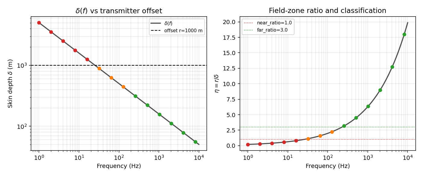
Skin depth and eta ratio versus frequency, coloured by near, transition, and far field classification — Left: the skin-depth curve crosses the fixed 1 km offset right where the colour turns from red (near) through orange (transition) to green (far). Right: the same crossing, read off (12) against its `near_ratio`/`far_ratio` thresholds. Both panels classify the same 14 frequencies identically, because they are the same computation viewed two ways.#

In pyCSAMT, source-effect and field-zone tools should therefore be treated as diagnostics. They help identify where a conventional MT-style workflow may be safe, questionable, or inappropriate – and, as above, they can flag a correction as recommended before a single apparent-resistivity curve is even plotted. See Field Zones: Near, Transition, And Far Field for the full treatment: the Bostick depth-based \(|k\cdot r|\) parameter pyCSAMT actually implements, the analytical near-field correction and Yan (2004) shadow-effect formulas, and a real CSAMT survey worked example rather than this synthetic transmitter comb.

3.8. Apparent Resistivity Is Not True Resistivity#

Apparent resistivity is the resistivity of a hypothetical uniform half-space that would produce the observed response at one frequency. It is not the actual resistivity at a single depth. For MT-like impedance data:

(13)#\[\rho_a(f) = \frac{|Z(f)|^2}{\mu_0 \omega}.\]

A pseudosection plots \(\rho_a\) or phase against station position and period/frequency. It is useful for quality control and qualitative geological inspection, but it is not a true cross-section. Main limitations include:

depth is only indirectly related to period;
apparent resistivity blends effects from a volume of Earth;
conductive and resistive targets have different sensitivity footprints;
topography, source effects, and static shift can distort patterns;
2-D and 3-D structures can produce responses that do not map vertically below each station.

For this reason, pyCSAMT documentation separates quick-look products from inversion products. Pseudosections are diagnostic and interpretive aids; resistivity models require a forward/inverse modelling step.

3.9. Dimensionality: 1-D, 2-D, And 3-D Earth Assumptions#

The interpretation method must match the geology closely enough to be useful. Dimensionality describes how resistivity varies in space.

Assumption	Resistivity structure	Typical use
1-D	\(\rho = \rho(z)\)	Layered Earth sounding, first-pass modelling, station-by-station inversion, synthetic tests.
2-D	\(\rho = \rho(x,z)\) and approximately invariant along strike.	Profile interpretation when geological strike is stable and station spacing is along a crossing line.
3-D	\(\rho = \rho(x,y,z)\)	Complex geology, strong lateral changes, non-profile surveys, source and topographic complexity.

Many CSAMT/AMT field projects start with 1-D or 2-D thinking because it is fast and interpretable. That does not mean the Earth is actually 1-D or 2-D. Phase tensor analysis, skew, tipper behavior, induction arrows, strike estimates, and residual patterns help decide whether a simplified inversion is defensible. This site-level classification is a different idea from Quasi-3-D forward modelling, which approximates a full 3-D response from 2-D slices for synthetic experiments – one describes what the recorded data actually look like, the other is a computational shortcut for generating synthetic data in the first place. Dimensionality, Distortion, And The Phase Tensor derives the phase tensor’s orientation and skew angles and works through a real 28-station example where the rule-based classifier labels the majority of station-periods 3-D.

3.10. Source Type And Data Interpretation#

A useful way to think about method choice is to ask: “What source generated the field I am interpreting?”

Natural-source MT/AMT:

source is not controlled by the operator;
plane-wave field assumption is central;
impedance tensor is the primary response;
remote reference and robust processing may be important;
weak natural signal intervals can limit data quality.

Controlled-source CSAMT/CSEM:

source location, orientation, waveform, and current are part of the experiment;
signal strength can be high and repeatable;
source geometry can contaminate MT-style apparent resistivity;
near field, transition field, and far field behavior must be checked;
full controlled-source modelling may be needed for rigorous inversion.

Time-domain TDEM:

source is switched off or changed in time;
measured response is a transient decay;
time gates replace frequency samples;
early times tend to sample shallower structure, later times deeper structure;
receiver coupling, gate timing, and transmitter waveform are central.

The same field project may combine methods. For example, TDEM can constrain shallow structure or static shift, AMT/CSAMT can provide profile-scale coverage, and MT can extend depth of investigation.

3.11. Coordinate And Component Conventions#

Most MT-style processing uses horizontal components:

\(E_x\), \(E_y\): horizontal electric fields;
\(H_x\), \(H_y\): horizontal magnetic fields;
\(H_z\): vertical magnetic field, used in tipper analysis.

Coordinate conventions must be tracked carefully. Rotating data changes the impedance tensor:

(14)#\[\mathbf{Z}' = \mathbf{R}(\theta) \mathbf{Z} \mathbf{R}^{T}(\theta),\]

where \(\mathbf{R}(\theta)\) is a horizontal rotation matrix. The goal is often to align data with geological strike or profile orientation. The details are covered in Impedance Tensor, but the practical message is simple: component labels only have meaning relative to a coordinate system.

3.12. Common Data Products#

pyCSAMT workflows commonly create or consume the following products.

Product	What it shows	How to use it
Apparent resistivity curve	\(\rho_a\) versus frequency or period at one station.	Inspect shifts, slopes, outliers, and frequency coverage.
Phase curve	Impedance phase versus frequency or period.	Identify conductive/resistive trends and dimensionality issues.
Pseudosection	Response plotted by station and period/frequency.	Quick-look lateral continuity and QC; not a true depth section.
Phase tensor plot	Distortion-resistant tensor geometry.	Dimensionality, strike, skew, and structural complexity.
Tipper/induction vectors	Vertical magnetic response to horizontal magnetic fields.	Lateral conductivity contrasts and 3-D effects.
Inversion model	Resistivity distribution produced by fitting data with a forward model.	Main quantitative interpretation product, subject to uncertainty.
Residual or misfit map	Difference between observed and predicted data.	Diagnose poor fits, noisy stations, model inadequacy, or source issues.

3.13. How pyCSAMT Uses These Concepts#

The theory pages are not isolated from the software. They explain why the workflow is organized the way it is.

pyCSAMT area	Theoretical connection
`pycsamt.seg` and `pycsamt.site`	Store station data, fields, impedance tensors, coordinates, and survey context.
`pycsamt.emtools`	Implements processing and diagnostic operations such as frequency editing, tensor analysis, static shift handling, source-effect diagnostics, and QC plots.
`pycsamt.iot`	Real-time and post-acquisition edge diagnostics, including the `classify_field_zones()` field-zone check used above.
`pycsamt.pipeline`	Chains theory-aware processing steps into reproducible workflows.
`pycsamt.models` and `pycsamt.inversion`	Prepare and interpret model-based inversion workflows such as Occam2D and ModEM.
`pycsamt.agents`	Help translate user requests into workflow plans, run diagnostics, and explain output products.
`pycsamt.app`	Provides desktop and web interfaces for the same processing concepts.

3.14. Practical Reading Of A Survey#

When approaching a new MT/AMT/CSAMT survey, a robust interpretation sequence is:

Confirm survey type, source type, coordinate system, station spacing, frequency/period band, and file format.
Inspect station metadata and frequency coverage before interpreting any pseudosection.
Check apparent resistivity and phase curves station by station.
For CSAMT, inspect field-zone and source-effect diagnostics (as above) before treating the data as MT-like impedance data.
Check static shift risk, especially in rugged near-surface geology or resistive/conductive shallow cover.
Evaluate dimensionality with phase tensors, skew, strike, tipper, and profile consistency.
Choose a model class: 1-D, 2-D, 3-D, or controlled-source forward/inverse modelling as required.
Interpret inversion results with residuals, RMS misfit, uncertainty, geology, and independent constraints.

This sequence is deliberately conservative. EM responses are subject to non-uniqueness – many different subsurface models can explain similar data. Good workflows make assumptions explicit and preserve enough QC information to revisit those assumptions later.

3.15. Common Interpretation Pitfalls#

The most common mistakes are conceptual rather than computational:

treating a pseudosection as a true geological section;
ignoring source effects in CSAMT data;
interpreting shifted apparent resistivity as a real layer without checking static shift;
assuming high-frequency data always mean shallow depth in every resistivity environment;
using a 2-D inversion when the data show strong 3-D behavior;
comparing stations without checking coordinate rotation and component convention;
trusting a low RMS misfit inversion without inspecting residual distribution and geological plausibility.

The purpose of pyCSAMT’s processing, pipeline, and agent layers is to make these checks repeatable.

3.16. References#

This overview is consistent with standard EM theory and MT/CSAMT practice, including the methodology references collected in References. Especially relevant entries include [WardHohmann1988], [Yan2004], [Chen2005], [Da2016], [WangLin2023], [Zhang2021], [deGrootHedlin1990], and [Kelbert2014].

3.17. Next Steps#

Continue with:

Impedance Tensor for tensor notation, apparent resistivity, phase, rotations, strike, and tipper;
Static Shift for near-surface galvanic distortion and correction strategies;
Inversion Concepts for model fitting, regularization, misfit, and non-uniqueness;
TDEM Basics for time-domain EM concepts.