
10. Inversion Concepts#
Electromagnetic inversion is the process of estimating a subsurface resistivity model from measured electromagnetic responses. In pyCSAMT, this idea appears in several places: the built-in inversion backend, the Occam2D and ModEM adapters, MARE2DEM helpers, pipeline presets, and AI-assisted agents that inspect configuration and outputs. All of them share the same scientific problem:
That arrow is not unique – this is exactly the non-uniqueness introduced formally later on this page. Many different resistivity distributions can produce similar apparent resistivity, phase, impedance, tipper, or transient decay curves. The role of inversion is therefore not only to fit the data, but to find a model that fits the data within credible errors while remaining geologically and numerically reasonable.
This page explains the concepts needed to read pyCSAMT inversion results and
to make good choices in pycsamt.inversion.config.InversionConfig,
Occam2D, ModEM, MARE2DEM, SimPEG, pyGIMLi, and pipeline workflows. Every
number quoted below comes from a single real builtin backend run kept
running throughout the page, not a hypothetical.
10.1. The Forward and Inverse Problems#
The forward problem predicts data from a known subsurface model. If \(m\) is the model parameter vector and \(F\) is the electromagnetic forward operator, the predicted data are
For magnetotelluric and CSAMT data, \(F\) solves Maxwell’s equations for the chosen source geometry, dimensionality, and boundary conditions, then extracts impedance-derived quantities such as apparent resistivity and phase – exactly (6) from CSAMT, AMT, and MT Overview, applied inside a forward model. For TDEM data, \(F\) predicts decay values at measured time gates.
The inverse problem starts with observed data and searches for a model:
where \(e\) represents noise, processing error, source effects, static shift, cultural coupling, dimensionality error, and other mismatch between the mathematical model and the real survey.
Because \(F\) is nonlinear for EM problems, inversion normally proceeds iteratively:
choose a starting model,
predict data from that model,
compare predicted and observed data,
update the model,
repeat until the data fit and model structure are acceptable.
10.2. Model Parameters#
Inversion does not usually solve directly for resistivity \(\rho\). It solves for a transformed parameter that is numerically more stable, commonly logarithmic resistivity or logarithmic conductivity:
with \(\sigma = 1/\rho\).
The logarithmic form has three advantages:
resistivity remains positive after exponentiation,
conductors and resistors are handled on a comparable relative scale,
smoothness penalties act on resistivity contrasts rather than absolute ohm-metre differences.
The model can be parameterized as:
1-D layers - each station is represented by a layered model whose resistivity varies only with depth, terminated by a half-space;
2-D sections - resistivity varies with profile distance and depth, but is assumed constant along strike;
3-D volumes - resistivity varies in all three spatial directions.
The correct parameterization is not simply the most detailed one. A 3-D model can be scientifically appropriate but expensive and poorly constrained if the survey geometry is sparse. A 1-D inversion can be robust and useful for sounding interpretation, but misleading near lateral contacts.
10.3. Data Vectors#
An inversion packs observations into a data vector \(d_{\mathrm{obs}}\). For EM workflows this vector may contain different components:
apparent resistivity \(\rho_a\);
phase \(\phi\);
real and imaginary impedance components;
TE, TM, or determinant-mode data;
tipper components;
TDEM gates;
CSEM responses for controlled-source workflows.
In pyCSAMT, component-aware error handling lives in
pycsamt.inversion.objective. The same conceptual data vector may be
represented as arrays, mappings, EDI-derived objects, Occam files, ModEM data
files, or pipeline products, but the inversion still sees weighted residuals.
pyCSAMT’s own EMData container is exactly
this: a plain frequencies/rho_a/phase record, seen below once a
real config is built from it.
10.4. Data Errors and Weights#
The data error \(\sigma_i\) says how much trust to place in observation \(i\). The normalized residual is
Small errors make a datum influential; large errors make it less influential. If errors are unrealistically small, the inversion will chase noise and processing artifacts. If errors are too large, the model may fit only the largest trends.
The weighted data misfit is usually written as
where \(W_d\) is commonly a diagonal matrix with entries \(1 / \sigma_i\).
pyCSAMT’s shared configuration exposes this idea through parameters such as
error_floor, phase_error, and backend-specific error_model options.
The default behavior is to use relative floors for amplitude-like quantities
and an absolute phase error in degrees for phase. Component masks can exclude
bad stations, frequencies, time gates, or individual samples from the
objective function.
10.4.1. Error Floors#
An error floor prevents the inversion from assigning excessive importance to values whose formal processing error is very small. A common apparent resistivity floor is
where \(f_\rho\) is a relative floor such as 0.05 for 5 percent.
For phase, a practical floor is often absolute:
In pyCSAMT, phase_error=3.0 means an absolute phase floor of 3 degrees
unless overridden by a backend-specific error model.
10.5. Objective Function#
A regularized inversion minimizes an objective function containing at least two terms:
Here \(\Phi_d\) is the data misfit, \(\Phi_m\) is the model penalty,
and \(\lambda\) controls the trade-off between fitting data and keeping
the model simple. Some backends expose this scalar as lambda, lam,
regularization_weight, or an internal cooling schedule.
The model selected by inversion is therefore not just “the model that fits best.” It is the model that fits the data with an acceptable structure under the chosen assumptions.
10.6. Regularization#
Regularization expresses what kind of model is preferred when the data do not uniquely determine every cell. Without regularization, many EM inversions are unstable because small data changes can produce large model changes.
Smooth regularization penalizes roughness:
In this expression:
\(m_{\mathrm{ref}}\) is a reference model;
\(D_x\) and \(D_z\) are finite-difference operators;
\(\alpha_s\) controls smallness relative to the reference model;
\(\alpha_x\) controls lateral smoothness;
\(\alpha_z\) controls vertical smoothness.
pyCSAMT’s pycsamt.inversion.regularization module uses the shared
vocabulary smooth, damped, blocky, and none. A smooth
penalty favors gradual changes. A damped penalty also pulls the solution
toward a reference model. A blocky penalty reduces the cost of sharp
edges and can be useful when the target is expected to contain contacts,
faults, or compact bodies.
Blocky regularization is often expressed using a robust norm, for example
where \(\epsilon\) prevents singular behavior near zero gradient. The result is less smooth than an \(L_2\) model, but still controlled.
10.7. The Trade-Off Parameter#
The trade-off parameter \(\lambda\) determines how expensive model structure is relative to data misfit.
Setting |
Typical behavior |
Risk |
|---|---|---|
\(\lambda\) too small |
Fits small data details and noise. |
Produces unstable or geologically implausible structure. |
\(\lambda\) balanced |
Fits data within errors and keeps only required structure. |
Requires diagnostics, not a single number. |
\(\lambda\) too large |
Produces very smooth or reference-like models. |
Misses real targets and underfits important data trends. |
Occam-style inversion searches for the simplest model that reaches a target misfit. Other backends may use a fixed \(\lambda\), a cooling schedule, or a line-search strategy. The practical question is the same: does the model fit the observations at the level justified by the errors?
10.8. RMS Misfit#
The normalized root-mean-square misfit is a compact summary of weighted residuals:
If the error model is realistic and residuals are approximately Gaussian, an RMS misfit near 1 means the prediction fits the data at about the expected noise level. This interpretation depends completely on the errors. An RMS of 0.4 may mean an excellent fit, but it may also mean the errors were inflated. An RMS of 3 may mean the model is wrong, but it may also indicate static shift, bad phase rotations, source effects, dead bands, or an underestimated error floor.
A real builtin 1-D MT run makes this concrete rather than hypothetical.
Five synthetic sounding points (a resistive-to-conductive trend typical of a
weathered layer over more resistive basement) are inverted for a 5-layer
model with smooth regularization:
>>> from pycsamt.inversion import InversionConfig, InversionWorkflow
>>> cfg = InversionConfig(
...     method="mt",
...     dimension="1d",
...     backend="builtin",
...     data={
...         "freqs": [1000.0, 316.0, 100.0, 31.6, 10.0],
...         "rho_a": [80.0, 95.0, 130.0, 210.0, 400.0],
...         "phase": [42.0, 44.0, 47.0, 50.0, 53.0],
...     },
...     n_layers=5,
...     error_floor=0.05,
...     phase_error=3.0,
...     regularization="smooth",
...     backend_options={
...         "regularization_weight": 1.0,
...         "alpha_z": 1.0,
...     },
... )
>>> result = InversionWorkflow(cfg).run()
>>> round(result.rms, 4)
2.4148
>>> result.status
'converged'
>>> len(result.history.records)
285
An RMS of 2.41, not 1, is the honest result for this particular 5-point sounding and these error settings – not adjusted to look better. Plotting the full 285-entry convergence history alongside the observed-versus-predicted curve shows both why it converged there and where the fit is weakest:
 1import matplotlib.pyplot as plt
 2
 3recs = result.history.records
 4iters = [r["iteration"] for r in recs]
 5rms_hist = [r["rms"] for r in recs]
 6
 7freqs = result.data.frequencies
 8rho_obs = result.data.rho_a
 9rho_pred = result.predicted.rho_a
10
11fig, axes = plt.subplots(1, 2, figsize=(10.5, 4.4))
12ax = axes[0]
13ax.plot(iters, rms_hist, color="#1f77b4", lw=1.8)
14ax.axhline(1.0, color="0.4", lw=1.0, ls="--", label="RMS = 1")
15ax.set(xlabel="Iteration", ylabel="RMS misfit",
16       title="Convergence history (builtin 1-D MT)")
17ax.legend(fontsize=8)
18ax.grid(True, alpha=0.3)
19
20ax = axes[1]
21ax.loglog(freqs, rho_obs, "o-", color="#1f77b4", label=r"observed $\rho_a$")
22ax.loglog(freqs, rho_pred, "s--", color="#d62728", label=r"predicted $\rho_a$")
23ax.set(xlabel="Frequency (Hz)", ylabel=r"$\rho_a$ ($\Omega\cdot$m)",
24       title=f"Data fit (final RMS={result.rms:.2f})")
25ax.legend(fontsize=8)
26ax.grid(True, which="both", alpha=0.3)
27fig.tight_layout()
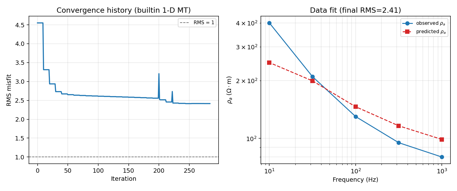
Left: RMS drops quickly from 4.55 to about 2.65 within the first 30 iterations, then creeps down slowly with two small real retries visible as spikes near iterations 200 and 220 – genuine optimizer behavior, not noise added for illustration. Right: the fit is good at the three highest frequencies but under-predicts the lowest-frequency (10 Hz) point by more than a factor of four, which is exactly what keeps the final RMS at 2.41 rather than nearer 1.#
Always inspect residuals by:
station,
frequency or time gate,
component,
mode,
profile position,
iteration.
A single global RMS can hide systematic failure. The right-hand panel above is a one-station illustration of exactly that: a single scalar RMS of 2.41 does not by itself say which frequency is driving the misfit, only the per-point comparison does. For example, a model may fit high frequencies well while missing deep low-frequency structure, or it may fit most stations while failing near one cultural-noise zone.
10.9. Dimensionality#
Choosing 1-D, 2-D, or 3-D inversion is a geologic decision, a survey-design decision, and a computational decision. Dimensionality here is the same concept as in CSAMT, AMT, and MT Overview, applied to the modelling choice rather than the data diagnostic.
Dimension |
Assumption |
Best use |
Main risk |
|---|---|---|---|
1-D |
Resistivity varies only with depth. |
Sounding curves, reconnaissance, layered settings, station-by-station checks. |
Lateral structure can be mapped into false vertical layering. |
2-D |
Resistivity varies along profile and depth, and is constant along strike. |
Profiles across contacts, faults, basins, aquifers, and mine corridors. |
Off-profile or 3-D bodies can distort the section. |
3-D |
Resistivity varies in all directions. |
Complex geology, grids of stations, non-2-D current systems. |
Requires more data, computation, and careful regularization. |
For CSAMT, dimensionality should also consider transmitter geometry and
source effects. The far-field MT approximation is not automatically valid in
controlled-source surveys – see CSAMT, AMT, and MT Overview’s
classify_field_zones() for a quantitative way
to check this before choosing a dimensionality. Dimensionality, Distortion, And The Phase Tensor covers
the phase-tensor skew/ellipticity classifier behind the 1-D/2-D/3-D counts
in more depth, plus the Groom-Bailey distortion correction that can be
applied before committing to a dimensionality.
10.10. Meshes, Cells, and Padding#
In 2-D and 3-D inversion, the earth is divided into cells forming a mesh. The mesh must be fine enough near stations and targets to represent the fields, but large enough at the boundaries to avoid artificial edge effects. Typical mesh decisions include:
horizontal cell size near stations;
vertical cell thickness near the surface;
growth rate with depth;
lateral and vertical padding;
topography representation;
air, ocean, or inactive cells;
fixed cells where the model should not change.
Mesh design affects inversion strongly. A very coarse mesh can smear targets. A very fine mesh can create unnecessary degrees of freedom and increase non-uniqueness. External engines such as Occam2D, ModEM, and MARE2DEM have their own mesh conventions; pyCSAMT adapters prepare or read those files and then return common result objects when possible.
10.11. Starting Models, Reference Models, and Bounds#
The starting model is the first model evaluated by the inversion. The reference model is the model used by damping or reference regularization. They may be identical, but they serve different purposes.
Starting models should be conservative. A homogeneous half-space or simple layered model is often better than an overly detailed guess. The goal is to help the optimizer begin in a plausible region, not to force the final answer.
Reference models are more interpretive. They are useful when independent information is credible, for example borehole resistivity, known water-table depth, a mapped conductive overburden, or a fixed seawater layer. When the reference model is uncertain, reduce its weight and let the data speak.
Bounds limit model parameters to plausible ranges. The config below is a
real InversionConfig – it does not run (run_external=False and no
Occam2D binary is invoked here), but every attribute is genuinely validated
and stored by the dataclass, including the bounds dictionary:
>>> bounds_cfg = InversionConfig(
...     method="csamt",
...     dimension="2d",
...     backend="occam2d",
...     data="survey.edi",
...     workdir="runs/occam2d_csamt",
...     error_floor=0.05,
...     phase_error=3.0,
...     regularization="smooth",
...     bounds={
...         "log10_rho": (-1.0, 5.0),
...     },
...     run_external=False,
... )
>>> bounds_cfg.bounds
{'log10_rho': (-1.0, 5.0)}
>>> bounds_cfg.backend, bounds_cfg.dimension, bounds_cfg.run_external
('occam2d', '2d', False)
In this example, the resistivity search is limited to \(10^{-1}\) to \(10^5\) ohm-m in log10 space. The exact bound syntax depends on the backend, but the concept is shared.
10.12. Backend Concepts in pyCSAMT#
pyCSAMT separates the common inversion vocabulary from backend-specific
file formats and executables, all addressable through one
inversion backend name on InversionConfig.
Backend or module |
Main role |
Conceptual emphasis |
|---|---|---|
|
Dependency-light local inversion for practical checks and examples. |
Shared data errors, weighted residuals, simple 1-D and stitched 2-D workflows. |
|
Adapter to Occam2D-style smooth 2-D inversion. |
Find the smoothest model that reaches a target misfit. |
|
Adapter to ModEM 2-D/3-D workflows. |
Modular EM inversion with covariance and smoothing controls. |
|
Optional scientific Python inversion backend. |
Flexible simulation, optimization, and regularization machinery. |
|
Optional inversion backend for geophysical modelling workflows. |
Regularized inversion with pyGIMLi’s lambda-style controls. |
|
File builders, runners, source management, logs, and result loaders for MARE2DEM. |
2.5-D finite-element modelling and Occam-style inversion. |
|
Repeatable survey-to-result orchestration. |
Configuration, steps, presets, output directories, and provenance. |
|
AI-assisted review and orchestration helpers. |
Configuration inspection, inversion guidance, report drafting, and quality-control summaries. |
10.12.1. Occam2D#
Occam inversion is based on a clear principle: among the models that fit the data to the requested level, choose the simplest one. In 2-D MT and CSAMT sections, simplicity is usually expressed as smoothness of the resistivity model. This is why Occam2D results often look geologically restrained rather than sharply blocky.
In pyCSAMT, the Occam2D backend is most useful when the user wants to prepare
or load a conventional Occam2D project while keeping the high-level
configuration in pycsamt.inversion.config.InversionConfig.
10.12.2. ModEM#
ModEM is designed for modular electromagnetic inversion, especially 3-D MT workflows. Its model, data, covariance, and control files make the inversion state explicit. The covariance file is conceptually part of the regularization: it describes smoothing behavior and inactive or special cells such as air and ocean.
In pyCSAMT, ModEM support is handled by dedicated model/data/covariance builders and an inversion backend adapter. The theory of the objective function remains the same, but the practical controls follow ModEM file conventions.
10.12.3. MARE2DEM#
MARE2DEM is a 2.5-D finite-element code for controlled-source EM, MT, and related data types. It is valuable when adaptive finite elements and MARE2DEM-compatible project files are required. pyCSAMT includes utilities for building input sets, managing the source/binary lifecycle, running the executable, parsing logs, and loading outputs.
For users, the important concept is that MARE2DEM is an external inversion engine. pyCSAMT helps prepare, launch, and interpret the workflow, but the physics and optimizer are provided by the MARE2DEM code.
10.13. Data Preparation Before Inversion#
Inversion quality is often determined before the first iteration. A robust workflow should check:
station locations, elevations, and profile order;
frequency overlap between stations;
dead bands and noisy frequencies;
impedance rotations and coordinate conventions;
TE/TM mode assignment for 2-D interpretation;
static shift in apparent resistivity;
phase wrapping or sign errors;
transmitter distance and source effects for CSAMT;
topography and known air/water layers;
realistic error floors and masks.
Static shift deserves special care. It can move apparent resistivity curves up or down with little phase change, creating false shallow resistivity structure – exactly the real L18PLT before/after comparison in Static Shift. See Static Shift and the static-shift correction tutorials before trusting shallow contrasts in CSAMT or MT inversion output.
10.14. Interpreting Residuals#
Residuals are often more informative than the final resistivity image. A good residual review asks:
Are residuals randomly distributed, or do they form patterns?
Do high residuals concentrate at a few stations?
Are low frequencies or high frequencies systematically misfit?
Does one component dominate the objective function?
Is the inversion fitting phase but missing apparent resistivity, or the reverse?
Do residuals improve with iterations, or stagnate early?
The right-hand panel in the RMS Misfit figure above is exactly this kind of review at its smallest scale: one station, one component, five frequencies, and the 10 Hz point immediately identifies itself as the dominant contributor to the RMS. Patterned residuals usually indicate that the assumptions are incomplete. Examples include a 1-D inversion applied to a 2-D contact, a 2-D inversion affected by off-profile structure, a CSAMT source effect treated as far-field MT, or a station whose impedance estimate is contaminated by cultural noise.
10.15. Uncertainty and Non-Uniqueness#
An inversion result is a constrained interpretation, not a direct photograph of the subsurface. Important uncertainty sources include:
measurement noise;
processing choices;
source geometry;
dimensionality assumptions;
mesh design;
regularization style;
starting and reference models;
geological equivalence between different resistivity structures.
Non-uniqueness means two models can be equivalent for the measured bandwidth but differ below the depth of investigation. A sharp target can be smeared by smooth regularization. A deep conductor can be poorly resolved if low-frequency data are noisy – sensitivity to that conductor is low even though the mesh may still display a cell there. A resistive basement may be resolved as a boundary depth, but not as a precise resistivity value; that boundary-depth-only recovery is a direct statement about the setup’s resolution.
For reporting, prefer language such as “a conductive zone is required by the data between stations A and B” over “the aquifer is exactly this shape.” Geological interpretation should combine resistivity with boreholes, geology, hydrology, geochemistry, or other geophysical methods when available.
10.16. From Resistivity to Geology#
Resistivity is sensitive to porosity, pore-fluid salinity, clay content, temperature, alteration, mineralization, saturation, and lithology. The same resistivity value can mean different things in different settings. For example, a conductor may indicate saline water, clay-rich sediments, graphitic shear zones, sulfides, or cultural infrastructure.
pyCSAMT therefore treats inversion and interpretation as separate stages. The
inversion model estimates a resistivity model. Interpretation
connects that model to geological or hydrogeological hypotheses. The
handoff is handled in modules such as pycsamt.interp and in
interpretation-oriented guides.
10.17. Practical pyCSAMT Workflow#
A typical pyCSAMT inversion workflow follows this sequence:
Load or convert field data.
Inspect impedance, apparent resistivity, phase, and station geometry.
Apply masks, error floors, and optional static-shift corrections.
Choose dimensionality and backend.
Build an
pycsamt.inversion.config.InversionConfig.Prepare or run the inversion backend.
Review RMS, residuals, iteration history, and warnings.
Plot the model and response fits.
Convert the result to an interpretation-ready resistivity model.
Document provenance and configuration.
Steps 5-8 are exactly the cfg/result pair already built in the RMS
Misfit section above – there is no separate synthetic version of this
workflow on this page. The recovered 5-layer model is real output, not a
placeholder:
>>> import numpy as np
>>> np.round(result.model.resistivities, 2)
array([103.3 , 239.41, 274.47,   8.52,  29.34])
>>> result.model.name
'builtin_1d'
For a production external run, the same high-level configuration would point
to an Occam2D, ModEM, or MARE2DEM working directory and executable settings,
following the bounds_cfg pattern shown above.
10.18. Common Pitfalls#
The following mistakes are common in EM inversion projects:
treating low RMS as proof that the geological model is correct;
using formal processing errors without realistic error floors;
ignoring static shift before interpreting shallow resistivity;
applying 1-D inversion to strongly 2-D or 3-D structure;
accepting a 2-D section without checking off-profile effects;
overinterpreting cells below the practical depth of investigation;
using a complex mesh without enough data to constrain it;
mixing coordinate conventions between data, mesh, and topography;
comparing apparent resistivity pseudosections directly to true resistivity sections;
reporting resistivity anomalies as lithology without independent support;
reading a single global RMS as the whole story – the worked example above needed the per-frequency panel, not just
result.rms, to see where the fit actually broke down.
10.19. Pre-Inversion Checklist#
Before running inversion, confirm:
the method is correct:
mt,amt,csamt,emap, ortdem;station coordinates and elevations are in consistent units;
frequencies or time gates are sorted and valid;
bad samples are masked instead of silently retained;
apparent resistivity and phase use the expected units;
the chosen dimensionality matches the survey geometry;
the starting model is simple and plausible;
regularization is appropriate for the target;
bounds are wide enough to avoid forcing the answer;
output and work directories are versioned or reproducible.
10.20. Post-Inversion Checklist#
After inversion, review:
final RMS and its relation to the error model;
residual maps by station, frequency, and component;
observed-versus-predicted response curves;
convergence history and objective function trend;
sensitivity of the result to starting model and regularization;
whether major anomalies persist under reasonable parameter changes;
whether the interpreted depth range is supported by the data bandwidth;
warnings, missing files, and backend-specific logs;
exported models and provenance metadata.
10.21. Next Steps#
For implementation details, see:
Inversion for runnable pyCSAMT inversion examples;
Pipeline System for repeatable pipeline execution;
Inversion API for the generated inversion API;
Agent Overview for AI-assisted workflow review;
Impedance Tensor for impedance and apparent-resistivity theory;
Static Shift for static-shift concepts.
10.22. References#
The objective-function and regularization concepts used here follow standard electromagnetic inversion practice, including Occam inversion [deGrootHedlin1990], ModEM [Kelbert2014], and EM method fundamentals [WardHohmann1988]. The interpretation cautions about resistivity and geologic targets are consistent with [Palacky1988].