
12. TDEM Basics#
Time-domain electromagnetic methods, often called TEM or TDEM, measure the earth’s transient response after a controlled transmitter current changes with time. In contrast to MT, AMT, and CSAMT, where the primary observations are frequency-domain impedances, TDEM records decay curves at discrete time gates. Early gates are mainly sensitive to shallow structure; later gates are influenced by progressively deeper currents.
pyCSAMT uses TDEM in three related ways:
reading and plotting field TDEM products such as TEMAVG and ZPLOT files;
converting TDEM soundings to MT-like impedance/EDI products when a workflow needs frequency-domain compatibility;
inverting TDEM decay data directly through the inversion API when the data vector contains
timesandvalues.
This page explains the physical concepts behind those workflows and the
practical choices users must document, illustrated throughout with a real
sounding from the bundled 55-station data/TEMAVG/JIANGSU survey rather
than invented numbers.
12.1. Transient Diffusion#
In a common ground TDEM survey, a loop transmitter carries a steady current. At switch-off, the primary magnetic field collapses. Faraday induction creates eddy currents in the ground, and those currents diffuse outward and downward while decaying with time. The receiver measures a secondary-field quantity, commonly voltage, \(\partial B_z/\partial t\), or \(\partial H_z/\partial t\).
The diffusion character of TDEM is central. A useful dimensional estimate is
where \(z\) is a characteristic investigation depth, \(\rho\) is resistivity, \(t\) is time after switch-off, and \(\mu_0\) is the magnetic permeability of free space – the same \(\mu_0\) documented in Physical And Geodetic Constants, and the same square-root-of-time-over-\(\mu_0\) shape as the frequency-domain skin depth in CSAMT, AMT, and MT Overview, with \(t\) standing in for \(1/f\). This is only a scale estimate, not a resolution guarantee. It says that later times and more resistive earth tend to sample larger depths.
The TDEM response is therefore not a direct depth log. It is a time series controlled by transmitter moment, receiver geometry, waveform, earth conductivity, and data processing.
12.2. What Is Measured#
TDEM instruments usually record receiver voltage over a sequence of off-time
windows. The data are then processed into gate-centred values. In pyCSAMT,
one sounding is represented by pycsamt.tdem.TEMSounding, whose main
fields are:
Field |
Meaning |
|---|---|
|
Centre times of the off-time measurement windows in seconds. |
|
Decay value at each gate. |
|
Units or normalization of the decay values: |
|
Transmitter current in amperes. |
|
Transmitter loop area and turns, used to compute magnetic moment. |
|
Receiver coil geometry, needed for raw-voltage normalization. |
|
Receiver position relative to the transmitter loop. |
|
Transmitter-current waveform used for transform corrections. |
|
Optional absolute uncertainty at each time gate. |
The transmitter magnetic moment is
where \(I\) is current, \(n_{\mathrm{tx}}\) is transmitter turns, and
\(A_{\mathrm{tx}}\) is transmitter area. A larger moment increases signal
amplitude and may improve late-time signal-to-noise, but it does not remove
the need for correct geometry and noise handling. A real JIANGSU station
shows every field at once, including the fact that data arrives as raw
"voltage" while dBdt() applies the instrument calibration to convert
it to the physical \(\partial B_z/\partial t\) used by every formula
below:
>>> from pycsamt.tdem import read_temavg_soundings
>>> soundings = read_temavg_soundings(
...     "data/TEMAVG/JIANGSU", component="Hz", pattern="*.AVG",
... )
>>> len(soundings)
2790
>>> s0 = next(s for s in soundings if s.station_name == "TEM100_100")
>>> s0.n_gates
25
>>> s0.data_type
'voltage'
>>> s0.current, s0.tx_area, s0.tx_turns
(10.0, 129600.0, 1)
>>> round(float(s0.data[0]), 4), round(float(s0.dBdt()[0]), 8)
(0.7165, 7.165e-05)
12.3. Decay Curves#
A TDEM sounding is normally inspected as a decay curve: response amplitude versus time. Depending on the instrument and processing, the plotted value may be signed or absolute, linear or logarithmic, voltage or normalized field derivative.
For a simple central-loop late-time response over a uniform half-space, \(|\partial B_z/\partial t|\) approximately follows a power-law decay:
The real decay curve for station TEM100_100 traces this power law closely
across four decades of time before flattening into a noise floor at the
latest gates – exactly the kind of departure the “Common Mistakes” section
below warns against over-interpreting:
 1import numpy as np
 2import matplotlib.pyplot as plt
 3
 4fig, ax = plt.subplots(1, 1, figsize=(6.0, 4.2))
 5ax.loglog(s0.time_gates * 1e3, np.abs(s0.dBdt()), "o-",
 6          color="#1f77b4", ms=4, lw=1.4)
 7ax.set(xlabel="Time (ms)", ylabel=r"$|\partial B_z/\partial t|$ (T/s)",
 8       title=f"Decay curve ({s0.station_name})")
 9ax.grid(True, which="both", alpha=0.3)
10fig.tight_layout()
(the saved figure combining this with the late-time transform appears below, in the Late-Time Transform section).
This motivates the late-time apparent-resistivity estimate used by many TEM
workflows. pyCSAMT’s own LateTimeTransform
implements the central-loop asymptotic response of a magnetic dipole source
over a uniform half-space (Ward & Hohmann 1988, eq. 4.96; Nabighian &
Macnae 1991):
This formula is built for an idealized central-loop configuration and late
times. It is useful for quality control and approximate transformation, but
it should not be mistaken for a full inversion. Deriving it by hand from
pycsamt.constants.MU_0 and the same station’s moment and dBdt()
reproduces the library’s own output exactly:
>>> import numpy as np
>>> from pycsamt.constants import MU_0
>>> from pycsamt.tdem import LateTimeTransform
>>> lt = LateTimeTransform(freq_convention="skin_depth", phase_mode="homogeneous")
>>> out = lt.transform(s0)
>>> rho_manual = (
...     s0.moment * MU_0 ** 2.5
...     / (10.0 * np.sqrt(np.pi) * np.abs(s0.dBdt()) * s0.time_gates ** 2.5)
... ) ** (2.0 / 3.0)
>>> np.allclose(rho_manual[::-1], out["rho_a"])
True
>>> round(float(rho_manual[0]), 2)
1691.21
The array has to be reversed ([::-1]) before comparing – see the
Pseudo-Frequency section below for why the transform’s own output is
ordered by ascending frequency (equivalently, descending time) rather than
by the sounding’s native ascending-time order.
12.4. Time Gates#
TDEM data are not sampled at every instant. Measurements are integrated over time gates, then represented by gate centres. Gate design controls what the survey can see.
Early gates:
are most sensitive to shallow structure;
can be affected by transmitter ramp, receiver saturation, and system response;
may contain strong cultural or capacitive noise;
require careful waveform correction when the ramp is not negligible.
Late gates:
carry deeper information;
often have lower signal-to-noise ratio;
are sensitive to stacking quality and background noise;
may become negative, unstable, or clipped after processing.
Do not invert gates blindly. Inspect the decay curve and mask gates that are outside the reliable signal band.
12.5. Waveforms#
The transmitter current does not always switch off instantaneously. pyCSAMT
models several waveform types in pycsamt.tdem.waveform:
Waveform |
Meaning |
When to use |
|---|---|---|
|
Ideal square-wave current with zero ramp time. |
Late-time processing when ramp effects are negligible. |
|
Linear current turn-off over |
Early-time processing where finite ramp matters. |
|
Half-sine current envelope. |
Systems whose transmitted pulse follows a sinusoidal envelope. |
|
User-supplied time/current samples. |
Instrument-specific waveform corrections. |
The switch-off waveform matters most when the first gates are close to the
ramp duration. If a gate centre \(t\) is much larger than the ramp time,
the ideal step approximation may be adequate. If \(t\) is comparable to
the ramp, ignoring waveform shape can bias shallow apparent resistivity and
transformed frequency-domain products. Station TEM100_100’s own
waveform field is unset (None) in the raw AVG file – a real
reminder that the Fourier transform discussed later on this page needs
waveform metadata that a bare AVG file does not always carry.
12.6. Central-Loop and Offset Geometry#
Many ground TDEM surveys use a central-loop or coincident-loop geometry, where the receiver is near the centre of the transmitter loop. Other surveys use offset-loop, in-loop, slingram, or moving-loop layouts. Geometry changes the amplitude and spatial sensitivity of the response.
pyCSAMT stores:
transmitter area and turns;
current;
receiver coil area and turns;
loop shape and dimensions;
receiver offset or 2-D receiver position.
For non-central-loop configurations, a geometry correction may be required.
The CLI conversion command exposes this as --no-geometry-correction to
disable the default in-loop correction when the user intentionally wants raw
or externally corrected values. Every JIANGSU sounding loaded above reports
loop_shape="square" with offset=0.0 – a genuine central-loop survey,
which is why the late-time transform above needed no geometry correction
iteration.
12.7. Apparent Resistivity#
TDEM apparent resistivity is a derived diagnostic, not a direct measurement. It asks: “What uniform half-space would produce this gate value under the assumed geometry?” The answer varies with time because the real earth is not normally a uniform half-space.
When plotted against time or pseudo-depth, apparent resistivity helps reveal:
conductive overburden;
resistive basement;
late-time conductors;
noisy gates;
inconsistent station responses;
bad normalization or geometry metadata.
But apparent resistivity does not uniquely identify geology. A conductor can come from clay, saline water, sulfides, graphite, cultural infrastructure, or some combination. Interpretation must use geology and independent constraints.
12.8. Pseudo-Frequency#
Some pyCSAMT workflows convert TDEM data to MT-like EDI files. This requires assigning an equivalent frequency to each time gate. A common convention is
This relation is a convention, not a physical statement that the time-domain
measurement is identical to a sinusoidal MT measurement at one frequency.
It is useful for approximate comparison, plotting, and frequency-domain
pipeline compatibility. Because (5) is a strictly
decreasing function of \(t\), mapping an ascending-time array to
pseudo-frequency and then sorting by ascending frequency reverses the gate
order – confirmed above for station TEM100_100, where the transform’s
first output frequency (13.04 Hz) corresponds to the last raw time gate
(12.2 ms), not the first.
pyCSAMT exposes pseudo-frequency choices through TDEM transforms and the CLI
option --freq-convention. Users should report the convention used when
TDEM data are converted to EDI or merged with frequency-domain products.
12.9. Late-Time Transform#
The late-time transform is fast and practical. It estimates apparent resistivity from the decay curve and then synthesizes an impedance magnitude at pseudo-frequency:
A phase must also be assigned to build a complex impedance. pyCSAMT exposes
phase modes such as "homogeneous" and "weidelt" in the TDEM
conversion workflow.
Plotting the decay curve alongside the transformed apparent resistivity for the same real station shows both the input and the output of (4) side by side:
 1import numpy as np
 2import matplotlib.pyplot as plt
 3
 4fig, axes = plt.subplots(1, 2, figsize=(10.0, 4.2))
 5ax = axes[0]
 6ax.loglog(s0.time_gates * 1e3, np.abs(s0.dBdt()), "o-",
 7          color="#1f77b4", ms=4, lw=1.4)
 8ax.set(xlabel="Time (ms)", ylabel=r"$|\partial B_z/\partial t|$ (T/s)",
 9       title=f"Decay curve ({s0.station_name})")
10ax.grid(True, which="both", alpha=0.3)
11
12ax = axes[1]
13ax.loglog(out["freq"], out["rho_a"], "s-", color="#d62728", ms=4, lw=1.4)
14ax.set(xlabel="Pseudo-frequency (Hz)", ylabel=r"$\rho_a$ ($\Omega\cdot$m)",
15       title="Late-time transform")
16ax.grid(True, which="both", alpha=0.3)
17fig.tight_layout()
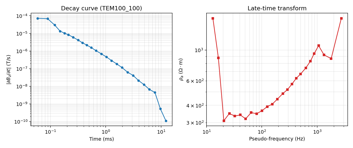
Left: the raw decay curve, a straight power-law line on log-log axes until the last two gates flatten into the noise floor. Right: the transformed \(\rho_a\) is not a clean sounding curve – it dips to about \(320\,\Omega\cdot\)m near 20-30 Hz then rises at both ends. The high-frequency (earliest-time) rise is exactly the symptom the next paragraph warns about: those gates are the least “late” in the sounding, where (4)’s late-time assumption is weakest.#
Use the late-time transform when:
data quality is sufficient and the target use is approximate frequency-domain compatibility;
the time gates are late enough for the approximation;
a fast survey-level conversion is more important than waveform-rigorous modelling.
Do not use it as proof that TDEM and MT data are interchangeable. The transformed product is an interpretation bridge.
12.10. Fourier Transform#
The more rigorous transform uses numerical Fourier integration to connect the time-domain response to frequency-domain quantities. It can include waveform effects and is better suited when early gates or non-ideal transmitter currents matter.
Use the Fourier transform when:
waveform metadata are reliable;
early-time information is important;
the transmitter waveform departs from an ideal step;
the transformed impedance will be used in a sensitive inversion or joint interpretation.
The cost is that it requires more complete acquisition metadata and is more
computationally involved – station TEM100_100 above, with
waveform=None, is exactly a case where only the late-time transform is
actually usable without first supplying a waveform model.
12.11. pyCSAMT Data Flow#
The TDEM subpackage follows a practical data flow:
read TEMAVG, ZPLOT, coordinate, or log files;
build
pycsamt.tdem.TEMSoundingobjects;attach geometry, waveform, station names, and coordinates;
inspect decay curves, sections, maps, and gate profiles;
optionally transform soundings to EDI collections;
pass transformed or direct TDEM data into inversion and interpretation workflows.
Step 3’s “coordinates” is worth checking rather than assuming. The station
positions for this survey live in a separate spreadsheet, Coordinate of
measuring point.xls; a plain *.AVG read does not carry them, but
pycsamt.tdem.read_temavg_survey() looks for that filename (or a plain
coordinates.csv) next to the AVG files and joins it automatically.
Reading a legacy .xls table this way needs the optional xlrd
dependency (pip install "pycsamt[docs]" or pip install xlrd); without
it the join is skipped and Coordinates reports none found instead of
raising, so always check this line rather than assuming the join succeeded:
$ pycsamt tdem info data/TEMAVG/JIANGSU
Survey root : data\TEMAVG\JIANGSU
AVG files   : 55
  TEM100  (1275 records)
  TEM1020  (1275 records)
  TEM1060  (1275 records)
  ...
Z files     : 55
LOG files   : 55
Coordinates : 5159 points  (with elevation)
Converting one real sounding to an EDI collection needs no coordinates to demonstrate the mechanics:
>>> from pycsamt.tdem import TEMtoEDI
>>> converter = TEMtoEDI(method="late_time", phase_mode="weidelt")
>>> collection = converter.transform(s0)
>>> len(collection)
1
>>> collection[0].station
'TEM100_100'
>>> collection[0].n_freq
25
Survey-folder conversion runs the same transform over every sounding in the directory at once:
>>> from pycsamt.tdem import transform_temavg_survey
>>> result = transform_temavg_survey(
...     "data/TEMAVG/JIANGSU",
...     component="Hz",
...     method="late_time",
...     freq_convention="skin_depth",
...     phase_mode="homogeneous",
...     return_collection=True,
... )
>>> result.n_soundings, result.n_results
(2790, 2790)
>>> len(result.collection)
2790
Every one of the 2790 soundings converts to a result here – unlike the
per-frequency masking seen for the static-shift factor tables in
Static Shift, nothing is silently dropped by this step. A production
run would add savepath="outputs/tdem_edi" to persist the collection as
EDI files instead of only building it in memory.
Command-line conversion follows the same pattern:
$ pycsamt tdem convert data/TEMAVG/JIANGSU --dry-run
Dry run - 2790 sounding(s) would be converted:
  TEM100_100
  TEM100_120
  TEM100_140
  ...

$ pycsamt tdem convert data/TEMAVG/JIANGSU \
    --output-dir outputs/tdem_edi \
    --method late_time \
    --component Hz
12.12. Plotting and QC#
Before conversion or inversion, plot the TDEM data. pyCSAMT provides plot helpers for:
decay curves;
transformed apparent resistivity;
TEMAVG sections;
ZPLOT sections;
station maps;
elevation profiles;
gate profiles;
compact dashboards.
The decay-curve panel already shown above is exactly
pycsamt.tdem.plot_decay() built by hand with plain Matplotlib, so the
one-call form is a direct substitute once coordinates are not needed:
>>> from pycsamt.tdem import plot_decay
>>> ax = plot_decay([s0])
>>> ax.get_title()
'TEM100_100'
When reviewing plots, look for:
sign reversals not explained by expected physics;
late-time noise floors;
early-time saturation or ramp artifacts;
stations with inconsistent amplitude after geometry normalization;
gates missing across many stations;
profile-aligned cultural features;
elevation or topography effects near station clusters.
12.13. TDEM Inversion#
TDEM can be inverted directly as a decay curve. In pyCSAMT’s inversion
configuration, this means method="tdem" and data containing time gates
and response values. The shared error model treats TDEM values with relative
and absolute floors, using configuration options such as error_floor and
backend-specific tdem_relative or tdem_absolute.
A minimal 5-gate synthetic decay, inverted the same way as the real MT sounding in Inversion Concepts, is an honest illustration of why the Post-Inversion Checklist there matters – the result below converges, but to an RMS far from 1, and the recovered top-layer resistivity (\(2\times10^5\,\Omega\cdot\)m) is not a value anyone should report without first checking residuals and error floors:
>>> from pycsamt.inversion import InversionConfig, InversionWorkflow
>>> cfg = InversionConfig(
...     method="tdem",
...     dimension="1d",
...     backend="builtin",
...     data={
...         "times": [1e-5, 3e-5, 1e-4, 3e-4, 1e-3],
...         "values": [2.0e-7, 5.0e-8, 1.2e-8, 2.5e-9, 6.0e-10],
...     },
...     n_layers=5,
...     error_floor=0.05,
...     regularization="smooth",
... )
>>> result = InversionWorkflow(cfg).run()
>>> round(result.rms, 4)
272.8703
>>> result.status
'converged'
status == "converged" here means the optimizer stopped changing the
model, not that the fit is good – rms=272.87 is a loud signal that this
5-point synthetic decay and these error settings do not constrain a 5-layer
model, exactly the “treating low RMS as proof” pitfall further down this
page, just illustrated with a bad fit instead of a good one.
Direct TDEM inversion avoids the interpretive step of synthesizing EDI files. Use it when the inversion backend supports the required TDEM physics and the survey geometry is represented adequately.
12.14. Combining TDEM With AMT, MT, or CSAMT#
TDEM is often combined with frequency-domain methods because they complement each other:
TDEM is strong for shallow conductive structure and static-shift control;
AMT/CSAMT may provide better frequency-domain continuity along profiles;
MT can extend sensitivity to greater depths;
transformed TDEM can help initialize or constrain frequency-domain interpretation.
However, the data are not identical measurements. When combining them:
keep original TDEM decay data;
record transform method and pseudo-frequency convention;
avoid over-weighting transformed TDEM points as if they were measured MT impedance;
check overlap consistency rather than forcing agreement;
document whether TDEM is used as direct inversion data, transformed EDI, or external constraint.
12.15. Noise and Error Floors#
TDEM noise is time dependent. Early gates can be affected by transmitter and receiver system response; late gates can approach the noise floor. A single percentage error is rarely perfect, but it is better than pretending all gates are exact.
The normalized residual for inversion is
For TDEM data, a practical error model combines relative and absolute floors:
The absolute floor prevents tiny late-time values from receiving excessive weight. The relative floor prevents high-amplitude gates from dominating only because their values are large.
12.16. Depth of Investigation#
TDEM depth of investigation is not a single number. It depends on:
transmitter moment;
receiver noise floor;
loop size and geometry;
earth resistivity;
gate range;
stacking and processing quality;
target geometry;
inversion regularization.
A late-time gate may not contain useful depth information if it is dominated by noise. Conversely, a shallow conductive layer can screen deeper structure, reducing the ability of later gates to resolve resistive basement.
A good report should state the reliable time range and avoid interpreting features below the supported depth range.
12.17. Common Mistakes#
Avoid these mistakes:
mixing milliseconds and seconds in
time_gates;using raw voltage without receiver area and turns;
forgetting transmitter current, area, or turns;
treating pseudo-frequency as measured MT frequency;
applying a late-time transform to early-time ramp-contaminated data – exactly the high-frequency upturn seen in the transformed curve above;
interpreting noisy late gates as deep conductors;
dropping sign information without documenting why;
converting to EDI without recording transform method and phase mode;
combining TDEM and AMT/MT data with incompatible weights;
reporting a smooth apparent-resistivity curve as a unique geological model.
12.18. Recommended Workflow#
A conservative TDEM workflow is:
Load survey files and coordinates.
Confirm units, current, loop area, turns, receiver geometry, and time units.
Plot decay curves and gate profiles.
Mask saturated, noisy, missing, or sign-unstable gates.
Choose whether the task needs direct TDEM inversion or EDI conversion.
If converting, select late-time or Fourier transform and record waveform assumptions.
Compare transformed products with AMT/MT/CSAMT only in compatible bands.
Invert with realistic relative and absolute error floors.
Interpret resistivity with geological constraints.
Archive original data, processed data, transform settings, and plots.
12.19. Reporting Checklist#
Include the following in reports or project metadata:
instrument and file type, such as TEMAVG or ZPLOT;
transmitter current, loop size, loop turns, and receiver geometry;
waveform type, base frequency, ramp time, or custom waveform file;
time-gate range and gates removed;
data type and units;
coordinate file and station naming;
transform method, pseudo-frequency convention, and phase mode;
error floors used for inversion;
plots of decay curves and gate/profile sections;
limitations on depth of investigation and geological interpretation.
12.20. Next Steps#
For implementation details, see:
pycsamt.tdem for the generated TDEM API;
TDEM Commands for command-line conversion and plotting;
Inversion Concepts for inversion objective functions and errors;
CSAMT, AMT, and MT Overview for method comparison with MT, AMT, and CSAMT.
12.21. References#
The transient diffusion and apparent-resistivity concepts follow standard TDEM references [NabighianMacnae1991] and [Christiansen2009]. General EM field theory follows [WardHohmann1988].