18.16. Building a Defensible 3-D AI Inversion Problem

A 3-D resistivity array is not automatically a 3-D inversion. A defensible result needs three connected objects: a geological volume, a Maxwell mesh that honours the acquisition and topography, and an optimizer whose predicted impedances reproduce observations not used to construct the model. This tutorial builds and inspects the first two with the current pycsamt.ai and pycsamt.forward.maxwell APIs, then applies the solver gate before training.

The distinction matters for the bundled L18PLT example. It is one profile, so all receiver coordinates lie close to a line. It can constrain an along-line section, but it cannot by itself identify arbitrary cross-line structure. Moreover, pycsamt.agents.Inv3DAgent currently returns a (station, layer) graph prediction. That object is useful for research and workflow testing; it is not a voxelwise, topographic 3-D Maxwell inversion. Consequently this page does not publish the former synthetic l18_ai3d_topography_block.png as an inversion result.

18.16.1. Start with the survey geometry

Load corrected EDIs through the canonical site contract and retain every station. Down-sampling may be useful for a quick software test, but station markers on a scientific figure must describe the data actually inverted.

>>> from pathlib import Path
>>> from pycsamt.emtools import ensure_sites
>>> from pycsamt.topo import extract_chainage, extract_elevation
>>> edi_dir = Path("data/AMT/WILLY_DATA/L18PLT")
>>> sites = ensure_sites(edi_dir, recursive=False, verbose=0).ordered()
>>> chain_km = extract_chainage(sites)
>>> elevation_m = extract_elevation(sites)
>>> len(sites), round(float(chain_km[-1]), 3)
(25, 4.029)
>>> (round(float(elevation_m.min()), 1), round(float(elevation_m.max()), 1))
(224.0, 274.0)

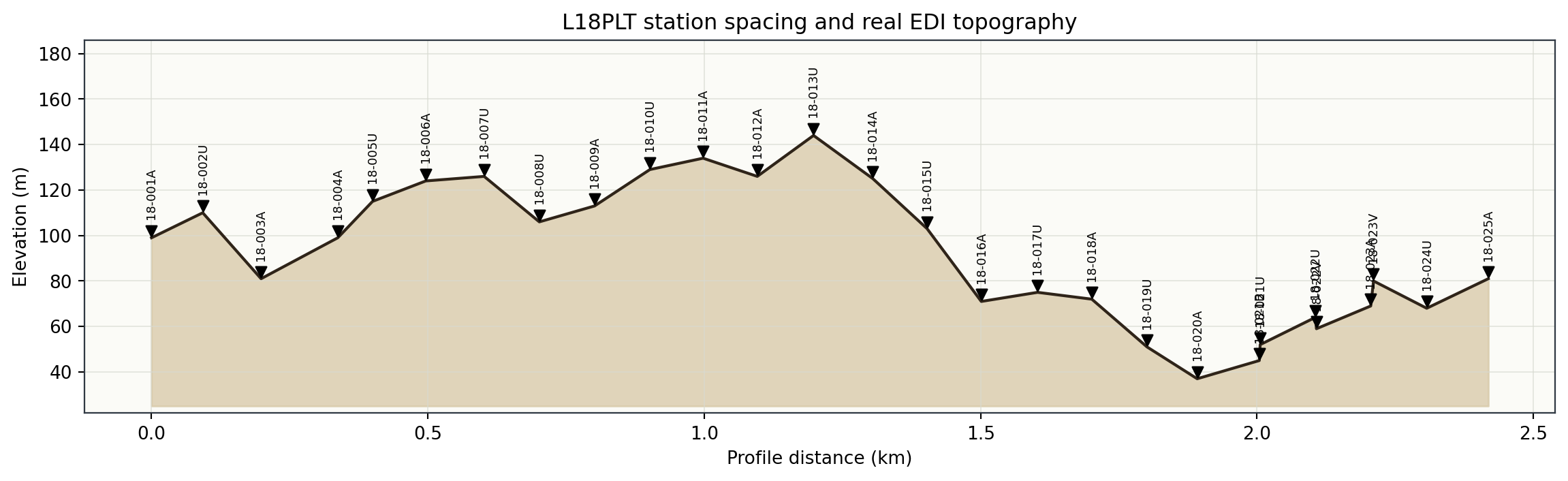
The clustered but nonuniform station spacing controls lateral resolution. The 50 m elevation range is also large enough that replacing the surface by a flat datum can move near-surface cells and receivers into the wrong physical region. Before attempting 3-D work, inspect the response curves, static-shift review, phase tensors, and corrected pseudosection exactly as described in AI Inversion From Corrected EDIs. Those diagnostics decide whether the data justify a 2-D approximation and reveal errors that no neural network can repair.

18.16.2. Define the 3-D geological hypothesis

The model below is a prior realization, not an inferred image of L18. It shows how the updated geology package expresses reproducible stratigraphy, spatially correlated heterogeneity, a dipping conductive body, and a terrain surface on one canonical (nz, ny, nx) grid.

>>> from pycsamt.ai.geology import (
...     ElectricalLayer, EllipsoidalLens, GaussianCorrelation,
...     GeologyGrid, TopographicSurface,
...     generate_layered_geology, insert_lenses,
... )
>>> grid = GeologyGrid.regular_3d(
...     nx=36, ny=24, nz=24,
...     dx_m=200, dy_m=200, dz_m=100,
...     x_origin_m=-3600, y_origin_m=-2400,
... )
>>> correlation = GaussianCorrelation(
...     1200, 180, length_y_m=800, azimuth_deg=25,
... )
>>> units = [
...     ElectricalLayer("weathered cover", 35, .10, correlation),
...     ElectricalLayer("resistive host", 900, .12, correlation),
...     ElectricalLayer("deep basement", 2200, .08, correlation),
... ]
>>> base = generate_layered_geology(
...     grid, units, [450, 1350], seed=41,
...     interface_relief_std_m=[70, 130],
...     interface_correlation=correlation,
...     minimum_thickness_m=150,
... )
>>> conductor = EllipsoidalLens(
...     "dipping conductor", 400, 900, 1100, 300, 8,
...     center_y_m=-100, radius_y_m=650,
...     azimuth_deg=30, dip_deg=18, transition_fraction=.20,
... )
>>> geology = insert_lenses(base, [conductor])
>>> grid.shape
(24, 24, 36)
>>> tuple(round(v, 1) for v in (
...     geology.resistivity_ohm_m.min(),
...     geology.resistivity_ohm_m.max(),
... ))
(8.0, 3878.7)

With \(\mathbf{x}=(x,y,z)\) and unit index \(k(\mathbf{x})\), the layer field is sampled in log-resistivity space,

(1)\[\log_{10}\rho(\mathbf{x}) = \log_{10}\bar{\rho}_{k(\mathbf{x})} + \sigma_{k(\mathbf{x})}\,g_{k(\mathbf{x})}(\mathbf{x}), \qquad C(\mathbf{h})= \exp\!\left[-\frac{1}{2}\sum_{q\in\{x,y,z\}} \left(\frac{h_q}{\ell_q}\right)^2\right].\]

Here the seed fixes each correlated field, while the correlation lengths \(\ell_q\) encode continuity rather than certainty. The lens then replaces or blends cells inside its rotated ellipsoidal support. Different plausible seeds, interfaces, and bodies should become an ensemble of priors; selecting only the realization that resembles the desired answer would bias validation.

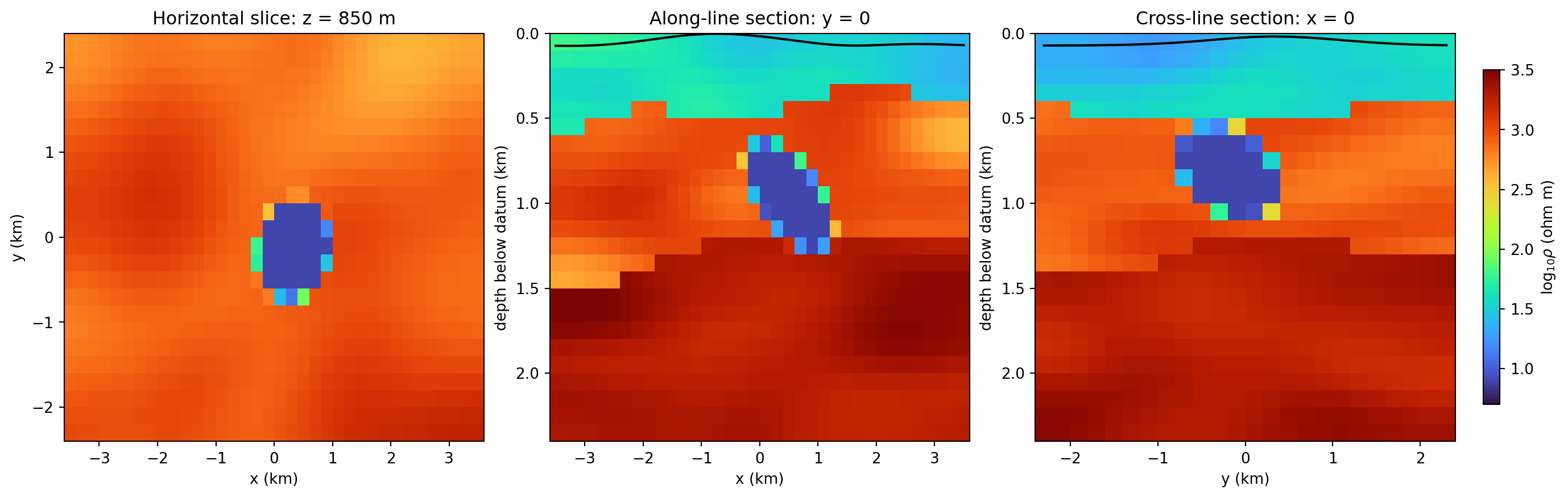
The central panel shows the expected along-line conductor, while the horizontal and cross-line panels expose information a single profile cannot determine. That unobserved cross-line extent is a prior assumption and must be reported as such. The black curves are the terrain depth relative to the highest surface point; cells above them belong to air, not geology.

The complete figure generator is exposed in the reproducibility section at the end of this tutorial, where it can be opened, copied, and run as one script.

18.16.3. Build the terrain-aware Maxwell mesh

The geology grid describes the core hypothesis. A forward solver additionally needs air cells, lateral and basal padding, conductivity, frequencies, and a terrain mask. pycsamt.forward.maxwell.build_solver_mesh() constructs that numerical model without silently changing the canonical array order.

>>> import numpy as np
>>> from pycsamt.forward.maxwell import MeshDesign, build_solver_mesh
>>> xx, yy = np.meshgrid(grid.x_m, grid.y_m)
>>> elevation = (
...     620 + 85 * np.exp(-((xx + 900) / 1500) ** 2
...                       - ((yy - 300) / 1100) ** 2)
...     - 45 * np.exp(-((xx - 1500) / 900) ** 2
...                       - ((yy + 500) / 700) ** 2)
...     + 18 * np.sin(xx / 1200)
... )
>>> topography = TopographicSurface(
...     grid, elevation, float(elevation.max()),
...     source="deterministic tutorial surface",
... )
>>> design = MeshDesign(
...     horizontal_padding_cells=4,
...     bottom_padding_cells=5,
...     air_layers=4,
...     padding_expansion=1.35,
... )
>>> solver_model = build_solver_mesh(
...     grid,
...     resistivity_ohm_m=geology.resistivity_ohm_m,
...     frequencies_hz=[100, 10, 1, .1],
...     topography=topography,
...     design=design,
... )
>>> solver_model.mesh.shape
(33, 32, 44)
>>> solver_model.quality.cell_count
46464
>>> len(solver_model.quality.warnings)
1

The executed topographic relief is 97.6 m. The mesh quality diagnostic uses the electromagnetic skin depth

(2)\[\delta(\rho,f)=\sqrt{\frac{\rho}{\pi\mu_0 f}},\]

and compares the smallest \(\delta\) over the requested frequency/model range with the largest core-cell width. A warning is not a cosmetic message: refine the affected direction or justify a backend-specific convergence study.

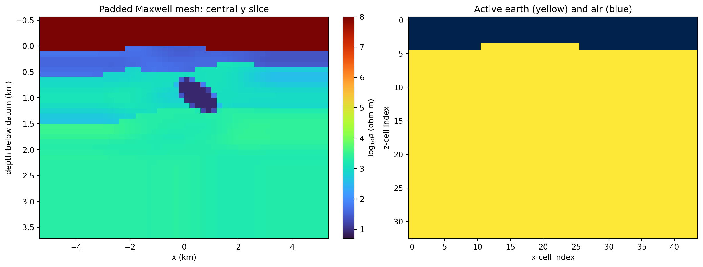
The left panel makes padding and highly resistive numerical air visible. The right panel verifies that the irregular surface becomes an explicit earth/air classification. Receivers must be placed consistently with that same datum; merely draping a finished image after inversion does not include topography in Maxwell’s equations.

18.16.4. Apply the backend gate before inversion

Compatibility is checked before expensive training because a physics loss is meaningful only if its forward operator supports the proposed problem. The bundled pycsamt.forward.maxwell.MT3DAdapter is deliberately labelled research-only. It supports a small uniform 3-D domain, but not nonuniform padding, inactive terrain cells, or this mesh size.

>>> from pycsamt.forward.maxwell import MT3DAdapter
>>> capability = MT3DAdapter().capabilities
>>> capability.dimensions
(3,)
>>> capability.maximum_cells
6000
>>> capability.supports_nonuniform_mesh, capability.supports_topography
(False, False)
>>> solver_model.quality.cell_count <= capability.maximum_cells
False

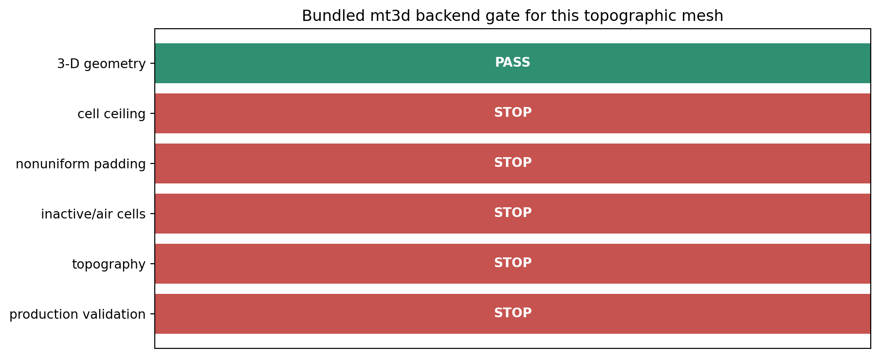
Only dimensionality passes for the proposed problem. Red STOP bars mean the solver must not be run by deleting padding, flattening terrain, or shrinking the mesh until it happens to fit. Instead, connect a validated external 3-D backend through pycsamt.forward.maxwell.ModEm3DAdapter, assess the exact pycsamt.forward.maxwell.MaxwellProblem, and preserve the compatibility report with the experiment.

18.16.5. What a complete external run must demonstrate

For observed impedance vector \(\mathbf{d}_{obs}\), model parameters \(\mathbf{m}\) (normally log conductivity), and a validated 3-D forward operator \(\mathcal{F}_{3D}\), training should minimize a declared objective such as

(3)\[\mathcal{J}(\mathbf{m}) = \left\|\mathbf{W}_d \left[\mathcal{F}_{3D}(\mathbf{m})-\mathbf{d}_{obs}\right]\right\|_2^2 +\lambda_s\|\mathbf{W}_s(\mathbf{m}-\mathbf{m}_{ref})\|_2^2 +\lambda_g\,\Phi_g(\mathbf{m}).\]

The first term is complex-impedance data misfit weighted by reported errors; the second controls spatial/model-reference departure; and \(\Phi_g\) expresses geological information without overriding data. A neural parameterization changes how \(\mathbf{m}\) is represented, not the need to evaluate \(\mathcal{F}_{3D}\) and its residuals.

Before promoting a volume, save and review all of the following:

• backend name/version, capability report, mesh and topography hashes;

• observed versus predicted impedance by station, frequency, and component;

• convergence histories for total and individual loss terms;

• synthetic recovery on held-out geological realizations;

• sensitivity or uncertainty maps, especially off the receiver line;

• comparison with a simpler 2-D/classical result and explicit failure cases.

The experimental graph command remains available in docs/scripts/run_ai_inv3d_candidate.py for software research. Run it in a separate output directory and treat pred_rho as a station-by-layer candidate, not as the geological volume built above. No candidate should be plotted as a 3-D inversion until the Maxwell and validation gates pass.

18.16.6. Reproduce the tutorial assets

Open the complete generator below to inspect or copy every operation used to construct the geology, topography, Maxwell mesh, capability gate, and figures. The panel is collapsed initially so the scientific narrative remains readable.

</>View and copy the complete tutorial-asset generatorClick to inspect and copy the complete code

#!/usr/bin/env python
# Author: LKouadio <etanoyau@gmail.com>
# License: LGPL-3.0
"""Generate reproducible geology and Maxwell-mesh figures for the 3-D tutorial."""

from __future__ import annotations

import sys
from pathlib import Path

import matplotlib

matplotlib.use("Agg")
import matplotlib.pyplot as plt
import numpy as np

ROOT = Path(__file__).resolve().parents[2]
sys.path.insert(0, str(ROOT))

from pycsamt.ai.geology import (  # noqa: E402
    ElectricalLayer,
    EllipsoidalLens,
    GaussianCorrelation,
    GeologyGrid,
    TopographicSurface,
    generate_layered_geology,
    insert_lenses,
)
from pycsamt.forward.maxwell import MeshDesign, MT3DAdapter, build_solver_mesh  # noqa: E402

IMAGE_DIR = ROOT / "docs/source/images/tutorials/essential_3d_ai_inversion"


def save(fig: plt.Figure, name: str) -> None:
    IMAGE_DIR.mkdir(parents=True, exist_ok=True)
    fig.savefig(IMAGE_DIR / name, dpi=190, bbox_inches="tight")
    plt.close(fig)


def build_model():
    grid = GeologyGrid.regular_3d(
        nx=36, ny=24, nz=24, dx_m=200, dy_m=200, dz_m=100,
        x_origin_m=-3600, y_origin_m=-2400,
    )
    corr = GaussianCorrelation(1200, 180, length_y_m=800, azimuth_deg=25)
    layers = [
        ElectricalLayer("weathered cover", 35, log10_std=0.10, heterogeneity=corr),
        ElectricalLayer("resistive host", 900, log10_std=0.12, heterogeneity=corr),
        ElectricalLayer("deep basement", 2200, log10_std=0.08, heterogeneity=corr),
    ]
    base = generate_layered_geology(
        grid, layers, [450, 1350], seed=41,
        interface_relief_std_m=[70, 130], interface_correlation=corr,
        minimum_thickness_m=150,
    )
    lens = EllipsoidalLens(
        "dipping conductor", center_x_m=400, center_y_m=-100,
        center_z_m=900, radius_x_m=1100, radius_y_m=650,
        radius_z_m=300, resistivity_ohm_m=8, azimuth_deg=30,
        dip_deg=18, transition_fraction=0.20,
    )
    geology = insert_lenses(base, [lens])
    xx, yy = np.meshgrid(grid.x_m, grid.y_m)
    elevation = (
        620 + 85 * np.exp(-((xx + 900) / 1500) ** 2 - ((yy - 300) / 1100) ** 2)
        - 45 * np.exp(-((xx - 1500) / 900) ** 2 - ((yy + 500) / 700) ** 2)
        + 18 * np.sin(xx / 1200)
    )
    topo = TopographicSurface(
        grid, elevation, float(np.max(elevation)), source="deterministic tutorial surface"
    )
    return grid, geology, topo


def plot_geology(grid, geology, topo) -> None:
    rho = np.log10(geology.resistivity_ohm_m)
    iz = int(np.argmin(abs(grid.z_m - 900)))
    iy = len(grid.y_m) // 2
    ix = len(grid.x_m) // 2
    fig, axes = plt.subplots(1, 3, figsize=(14.4, 4.5), constrained_layout=True)
    kw = dict(cmap="turbo", vmin=0.7, vmax=3.5, shading="auto")
    im = axes[0].pcolormesh(grid.x_m / 1000, grid.y_m / 1000, rho[iz], **kw)
    axes[0].set(title=f"Horizontal slice: z = {grid.z_m[iz]:.0f} m", xlabel="x (km)", ylabel="y (km)")
    axes[1].pcolormesh(grid.x_m / 1000, grid.z_m / 1000, rho[:, iy, :], **kw)
    axes[1].plot(grid.x_m / 1000, topo.surface_depth_m[iy] / 1000, color="black", lw=1.5)
    axes[1].invert_yaxis(); axes[1].set(title="Along-line section: y = 0", xlabel="x (km)", ylabel="depth below datum (km)")
    axes[2].pcolormesh(grid.y_m / 1000, grid.z_m / 1000, rho[:, :, ix], **kw)
    axes[2].plot(grid.y_m / 1000, topo.surface_depth_m[:, ix] / 1000, color="black", lw=1.5)
    axes[2].invert_yaxis(); axes[2].set(title="Cross-line section: x = 0", xlabel="y (km)", ylabel="depth below datum (km)")
    fig.colorbar(im, ax=axes, shrink=.82, pad=.02, label=r"$\log_{10}\rho$ (ohm m)")
    save(fig, "essential3d_geology_volume_slices.png")


def plot_mesh(grid, geology, topo):
    model = build_solver_mesh(
        grid, resistivity_ohm_m=geology.resistivity_ohm_m,
        frequencies_hz=[100, 10, 1, .1], topography=topo,
        design=MeshDesign(horizontal_padding_cells=4, bottom_padding_cells=5, air_layers=4),
    )
    sigma = model.conductivity_s_m
    iy = sigma.shape[1] // 2
    fig, axes = plt.subplots(1, 2, figsize=(12.8, 4.8), constrained_layout=True)
    x = model.mesh.cell_centres_m["x"] / 1000
    z = model.mesh.cell_centres_m["z"] / 1000
    im = axes[0].pcolormesh(x, z, np.log10(1 / sigma[:, iy, :]), cmap="turbo", shading="auto", vmin=.7, vmax=8)
    axes[0].invert_yaxis(); axes[0].set(title="Padded Maxwell mesh: central y slice", xlabel="x (km)", ylabel="depth below datum (km)")
    axes[1].imshow(model.earth_mask[:, iy, :], aspect="auto", origin="upper", cmap="cividis")
    axes[1].set(title="Active earth (yellow) and air (blue)", xlabel="x-cell index", ylabel="z-cell index")
    fig.colorbar(im, ax=axes[0], label=r"$\log_{10}\rho$ (ohm m)")
    save(fig, "essential3d_maxwell_mesh.png")
    return model


def plot_gate(model):
    cap = MT3DAdapter().capabilities
    checks = [
        ("3-D geometry", 3 in cap.dimensions),
        ("cell ceiling", model.quality.cell_count <= cap.maximum_cells),
        ("nonuniform padding", cap.supports_nonuniform_mesh),
        ("inactive/air cells", cap.supports_inactive_cells),
        ("topography", cap.supports_topography),
        ("production validation", False),
    ]
    fig, ax = plt.subplots(figsize=(9.4, 3.8), constrained_layout=True)
    y = np.arange(len(checks)); ok = np.array([v for _, v in checks])
    ax.barh(y, np.ones_like(y), color=np.where(ok, "#2f8f72", "#c6534f"))
    ax.set_yticks(y, [name for name, _ in checks]); ax.set_xlim(0, 1); ax.set_xticks([]); ax.invert_yaxis()
    for yi, value in zip(y, ok): ax.text(.5, yi, "PASS" if value else "STOP", ha="center", va="center", color="white", weight="bold")
    ax.set_title("Bundled mt3d backend gate for this topographic mesh")
    save(fig, "essential3d_backend_gate.png")


def main() -> int:
    grid, geology, topo = build_model()
    plot_geology(grid, geology, topo)
    model = plot_mesh(grid, geology, topo)
    plot_gate(model)
    print("geology shape:", grid.shape)
    print("resistivity range (ohm m):", f"{geology.resistivity_ohm_m.min():.1f}", f"{geology.resistivity_ohm_m.max():.1f}")
    print("topographic relief (m):", f"{topo.relief_m:.1f}")
    print("Maxwell mesh shape:", model.mesh.shape)
    print("Maxwell cells:", model.quality.cell_count)
    print("mesh warnings:", len(model.quality.warnings))
    print("mt3d maximum cells:", MT3DAdapter().capabilities.maximum_cells)
    return 0


if __name__ == "__main__":
    raise SystemExit(main())

Run the copied repository script from the project root:

python docs/scripts/generate_tutorial_essential_3d_ai_inversion.py

Executed output:

geology shape: (24, 24, 36)
resistivity range (ohm m): 8.0 3878.7
topographic relief (m): 97.6
Maxwell mesh shape: (33, 32, 44)
Maxwell cells: 46464
mesh warnings: 1
mt3d maximum cells: 6000

Continue with Solver-neutral Maxwell contracts for backend contracts, Correlated geological priors for richer prior ensembles, Training AI inversion models for experiment control, and Recovery, residual, and OOD diagnostics before reporting a scientific inversion.

Edit build_model() with your own grid geometry and layer resistivities to adapt this script