
18.6. Condition an MT Line With Tipper and Rotation#
This tutorial builds an auditable pre-inversion workflow for the KAP03 long-period MT line, which has both full impedance tensors and tipper data. The 26 sites form the southwest–northeast KAP03 profile of the Southern African Magnetotelluric Experiment (SAMTEX):
data/MT/kap03lmt_edis
The MTNet KAP03 data page documents the acquisition and contamination from the DC railway and mine power around KAP127–KAP145. Users must acknowledge the SAMTEX Consortium as required by the SAMTEX distribution page. Regional context and inversion sensitivity are discussed by Evans et al. (2011) and the ModEM/jif3D comparison of Moorkamp et al. (2022).
The aim is to make the processing decisions visible before inversion:
inspect raw tensor curves and tipper response;
identify weak frequency rows;
drop demonstrably weak rows and repair only isolated outliers;
inspect static-shift factors without automatically applying them;
estimate strike and plot phase tensors;
rotate impedance and tipper into a consistent frame.
This is an advanced tutorial. It deliberately avoids a single “automatic clean” button because MT conditioning is interpretive: every destructive or scaling operation should leave a trace in a table or figure.
18.6.1. Recommended Order#
The processing order used here is:
load the KP EDI line;
promote
DEFINEMEAScoordinates and attach sourced DEM elevations;plot raw
Zxx,Zxy,Zyx,Zyyapparent resistivity and phase;plot raw tipper components;
build station and frequency confidence tables;
drop low-confidence frequency rows from impedance and tipper together;
apply a conservative Hampel outlier filter;
estimate static-shift factors as a diagnostic and decide whether to use them;
estimate strike and plot phase tensor ellipses;
rotate impedance and tipper, export, reload, and validate.
18.6.2. Load the KP Line#
>>> from pathlib import Path
>>> from pycsamt.api import read_edis
>>> edi_dir = Path("data/MT/kap03lmt_edis")
>>> survey = read_edis(edi_dir, recursive=False, strict=True, progress=False)
>>> sites = survey.collection
>>> print(survey.summary())

APIFrame: edi_survey_summary
kind: edi.summary
shape: 26 rows x 6 columns
columns: station, path, n_freq, tipper, spectra, ts
numeric: 1 columns
missing: 0.0%
source: data/MT/kap03lmt_edis
Every loaded KP station has tipper rows in this sample:
>>> print(survey.summary().to_pandas()[["station", "n_freq", "tipper", "spectra"]].head(6).to_string(index=False))
station  n_freq  tipper  spectra
 kap103      20    True    False
 kap106      20    True    False
 kap109      18    True    False
 kap112      20    True    False
 kap115      20    True    False
 kap118      20    True    False
18.6.3. Recover Coordinates and Add Sourced Topography#
The EDI HEAD locations are empty and the original elevation values are
zero, but each DEFINEMEAS block carries REFLAT and REFLONG. The
generator promotes those coordinates and joins the cached
data/MT/kap03_topography_open_meteo.csv table. It was queried on
2026-08-03 with the Open-Meteo elevation API and records the service URL,
retrieval date, coordinate source, and elevation for every station.
>>> from pycsamt.site.utils import set_coords
>>> topo = pd.read_csv("data/MT/kap03_topography_open_meteo.csv").set_index("station")
>>> for site in sites:
...     dm = site.get_section("definemeas")
...     row = topo.loc[site.station]
...     assert abs(float(dm.reflat) - row.latitude) < 1e-5
...     assert abs(float(dm.reflong) - row.longitude) < 1e-5
...     set_coords(site, lat=dm.reflat, lon=dm.reflong,
...                elev=row.elevation_m, inplace=True)
>>> print(len(topo), topo.elevation_m.min(), topo.elevation_m.max())
26 473 1535
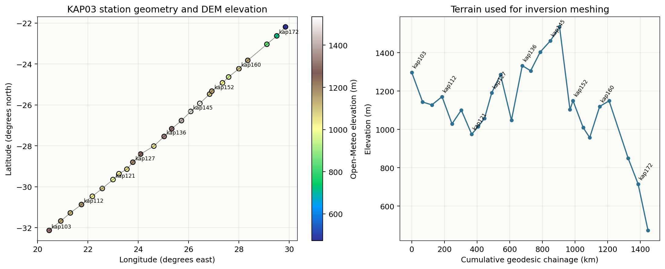
The recovered profile is approximately 1,447 km long. DEM elevation rises from 1,298 m at KAP103 to 1,535 m at KAP148 before falling to 473 m at KAP175. These remotely sampled elevations are not field differential-GNSS observations; terrain resolution and vertical-datum uncertainty belong in the near-surface mesh sensitivity analysis.#
The coordinate-validation and topography-injection step that produced the distances and elevations above:
View coordinate validation and topography injection codeClick to inspect and copy the complete code
 1def _inject_coordinates_topography(sites) -> pd.DataFrame:
 2    """Promote EDI DEFINEMEAS coordinates and cached DEM elevations."""
 3    from pycsamt.site.utils import set_coords
 4
 5    topo = pd.read_csv(TOPO_CSV)
 6    lookup = topo.set_index("station")
 7    rows = []
 8    for site in sites:
 9        ed = _edi(site)
10        dm = ed.get_section("definemeas")
11        row = lookup.loc[ed.station]
12        lat = float(dm.reflat)
13        lon = float(dm.reflong)
14        if abs(lat - float(row.latitude)) > 1e-5 or abs(lon - float(row.longitude)) > 1e-5:
15            raise ValueError(f"{ed.station}: cached coordinates disagree with DEFINEMEAS")
16        set_coords(ed, lat=lat, lon=lon, elev=float(row.elevation_m), inplace=True)
17        rows.append((ed.station, lat, lon, float(row.elevation_m)))
18    return pd.DataFrame(rows, columns=["station", "latitude", "longitude", "elevation_m"])
The map and terrain-profile figure itself comes from:
View the executed map and terrain-profile plotting codeClick to inspect and copy the complete code
 1def _plot_topography(coords: pd.DataFrame) -> None:
 2    lat = np.deg2rad(coords.latitude.to_numpy())
 3    lon = np.deg2rad(coords.longitude.to_numpy())
 4    dlat, dlon = np.diff(lat), np.diff(lon)
 5    a = np.sin(dlat / 2) ** 2 + np.cos(lat[:-1]) * np.cos(lat[1:]) * np.sin(dlon / 2) ** 2
 6    segment_km = 2 * 6371.0088 * np.arcsin(np.sqrt(a))
 7    distance = np.r_[0.0, np.cumsum(segment_km)]
 8    coords["chainage_km"] = distance
 9
10    fig, axes = plt.subplots(1, 2, figsize=(12.0, 4.8), constrained_layout=True)
11    sc = axes[0].scatter(coords.longitude, coords.latitude, c=coords.elevation_m,
12                         cmap="terrain", edgecolor="k", s=38)
13    axes[0].plot(coords.longitude, coords.latitude, "k-", lw=0.7, alpha=0.5)
14    for row in coords.iloc[::3].itertuples():
15        axes[0].annotate(row.station, (row.longitude, row.latitude), fontsize=7,
16                         xytext=(3, 3), textcoords="offset points")
17    axes[0].set(xlabel="Longitude (degrees east)", ylabel="Latitude (degrees north)",
18                title="KAP03 station geometry and DEM elevation")
19    fig.colorbar(sc, ax=axes[0], label="Open-Meteo elevation (m)")
20    axes[1].plot(distance, coords.elevation_m, "o-", ms=4, color="#2f6f8f")
21    for row in coords.iloc[::3].itertuples():
22        axes[1].annotate(row.station, (row.chainage_km, row.elevation_m),
23                         fontsize=7, rotation=55, xytext=(0, 6), textcoords="offset points")
24    axes[1].set(xlabel="Cumulative geodesic chainage (km)", ylabel="Elevation (m)",
25                title="Terrain used for inversion meshing")
26    for ax in axes:
27        _style_axis(ax)
28    _save(fig, "kp_coordinates_topography.png")
18.6.4. Plot Raw Tensor Curves#
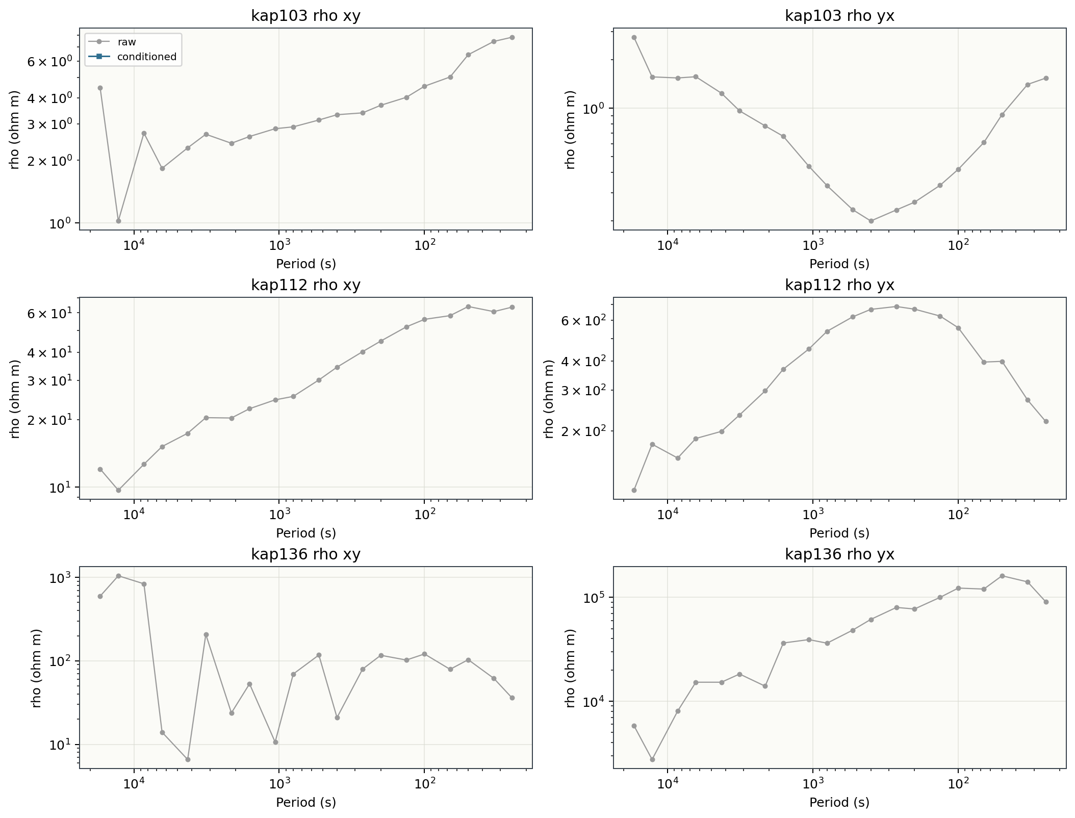
Before removing frequencies or scaling tensors, plot the raw components. The
off-diagonal components Zxy and Zyx normally carry the TE/TM response,
while the diagonal components Zxx and Zyy reveal 3-D effects, noise,
or rotation issues.
For angular frequency \(\omega=2\pi f\), the plotted quantities are \(\rho_{a,ij}=|Z_{ij}|^2/(\mu_0\omega)\) and \(\phi_{ij}=\operatorname{atan2}(\Im Z_{ij},\Re Z_{ij})\). Thus the apparent resistivity is amplitude-sensitive, whereas phase describes the complex response angle. The helper evaluates these expressions without changing the EDI objects:
>>> stations_to_plot = ["kap103", "kap112", "kap136", "kap169"]
>>> [(s.station, len(s.Z.freq)) for s in sites if s.station in stations_to_plot]
[('kap103', 20), ('kap112', 20), ('kap136', 20), ('kap169', 20)]
The generated figures show that this line is not a simple two-component data set; diagonal terms and phase behavior need to be reviewed before rotation.
>>> from pycsamt.emtools import plot_response_tipper
>>> fig = plot_response_tipper(
...     sites, stations=stations_to_plot, components=("xy", "yx"),
...     raw=True, ncols_groups=2, show_error_bars=True,
...     show_tipper_error_bars=True, recursive=False,
... )
>>> len(fig.axes)
32
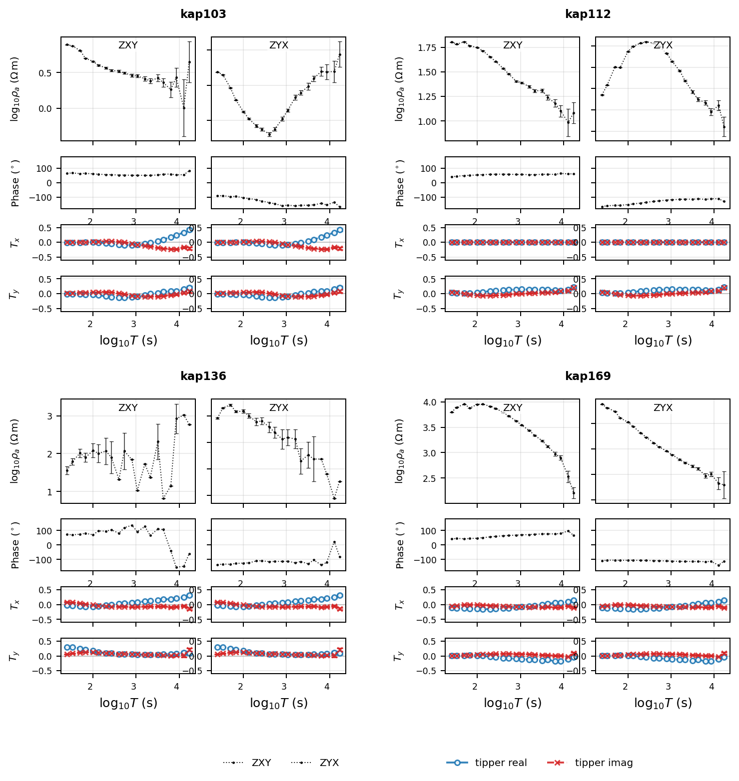
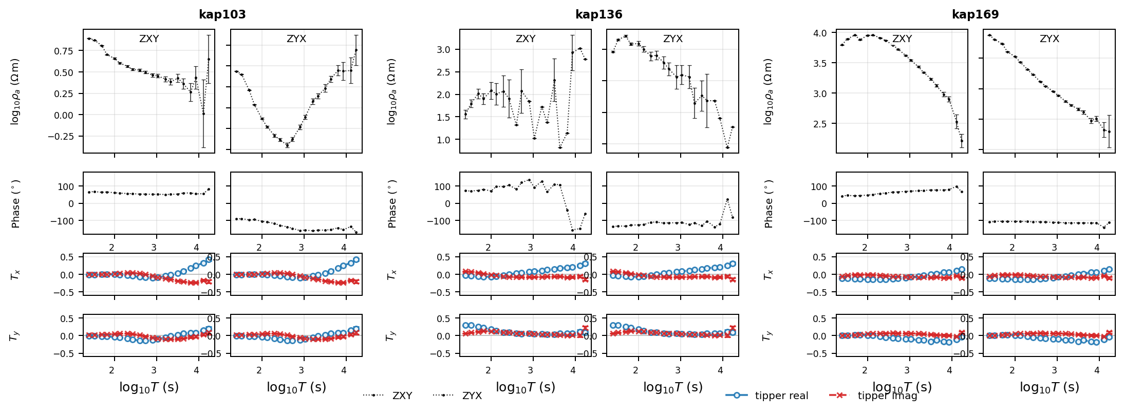
KAP136 lies within the railway/mine-power interval identified by MTNet and is therefore retained as a deliberately difficult example. Its irregular curves must not be smoothed merely to resemble its neighbours.
View the executed plot_response_tipper wrapperClick to inspect and copy the complete code
 1def _plot_raw_tensor(sites) -> None:
 2    """Use the public response API for raw rho, phase, and tipper."""
 3    from pycsamt.emtools import plot_response_tipper
 4
 5    fig = plot_response_tipper(
 6        sites, stations=STATIONS, components=("xy", "yx"), raw=True,
 7        ncols_groups=2, show_error_bars=True, show_tipper_error_bars=True,
 8        recursive=False,
 9    )
10    _save(fig, "kp_raw_response_tipper.png")
18.6.5. Plot Tipper Components#
Tipper data help identify lateral conductivity gradients and 3-D structure.
The KP EDI files store the tipper container as site.Tip:
>>> site = next(s for s in sites if s.station == "kap103")
>>> site.Tip.tipper.shape, site.Tip.freq[[0, -1]]
((20, 1, 2), array([4.00000e-02, 5.85938e-05]))
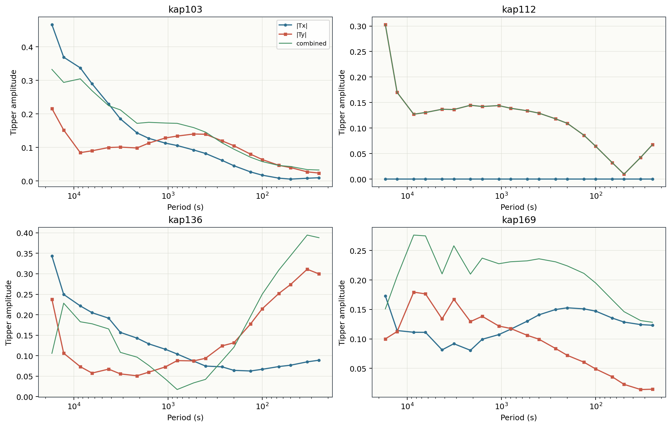
The tipper is a complex horizontal vector relating vertical to horizontal magnetic field. Large or rapidly changing amplitudes point to lateral conductivity gradients, but may also expose cultural noise. Because tipper and impedance share frequencies here, every later row rejection and rotation is applied to both.
View the executed raw tipper plotting codeClick to inspect and copy the complete code
 1def _plot_tipper(sites) -> None:
 2    """Use the public tipper-component API on three representative sites."""
 3    from pycsamt.emtools import plot_tipper_components
 4
 5    fig, axes = plt.subplots(1, 3, figsize=(13.0, 4.2), constrained_layout=True)
 6    for ax, station in zip(axes, ["kap103", "kap136", "kap169"]):
 7        plot_tipper_components(
 8            [_get_site(sites, station)], kind=("real", "imag"),
 9            axis="period", recursive=False, ax=ax,
10        )
11        ax.set_title(station)
12    _save(fig, "kp_raw_tipper_components.png")
18.6.6. Build QC Tables#
Use station-level and frequency-level tables before deciding what to suppress:
>>> from pycsamt.emtools import (
...     build_qc_table,
...     frequency_confidence_table,
...     station_confidence_table,
... )

>>> qc = build_qc_table(
...     sites,
...     include_skew=True,
...     recursive=False,
...     api=True,
... ).to_pandas(copy=True)

>>> station_ci = station_confidence_table(
...     sites,
...     method="composite",
...     recursive=False,
...     api=True,
... ).to_pandas(copy=True)

>>> freq_ci = frequency_confidence_table(
...     sites,
...     method="composite",
...     ci_hi=0.9,
...     ci_lo=0.5,
...     recursive=False,
...     api=True,
... ).to_pandas(copy=True)
>>> len(freq_ci), int((freq_ci.confidence < 0.5).sum())
(518, 30)
Example station QC:
station  n_freq  n_tip  frac_ok  snr_med  skew_med
 kap103      20     20    1.000   36.494     2.435
 kap106      20     20    1.000   33.926     4.761
 kap109      18     18    1.000   65.851     1.705
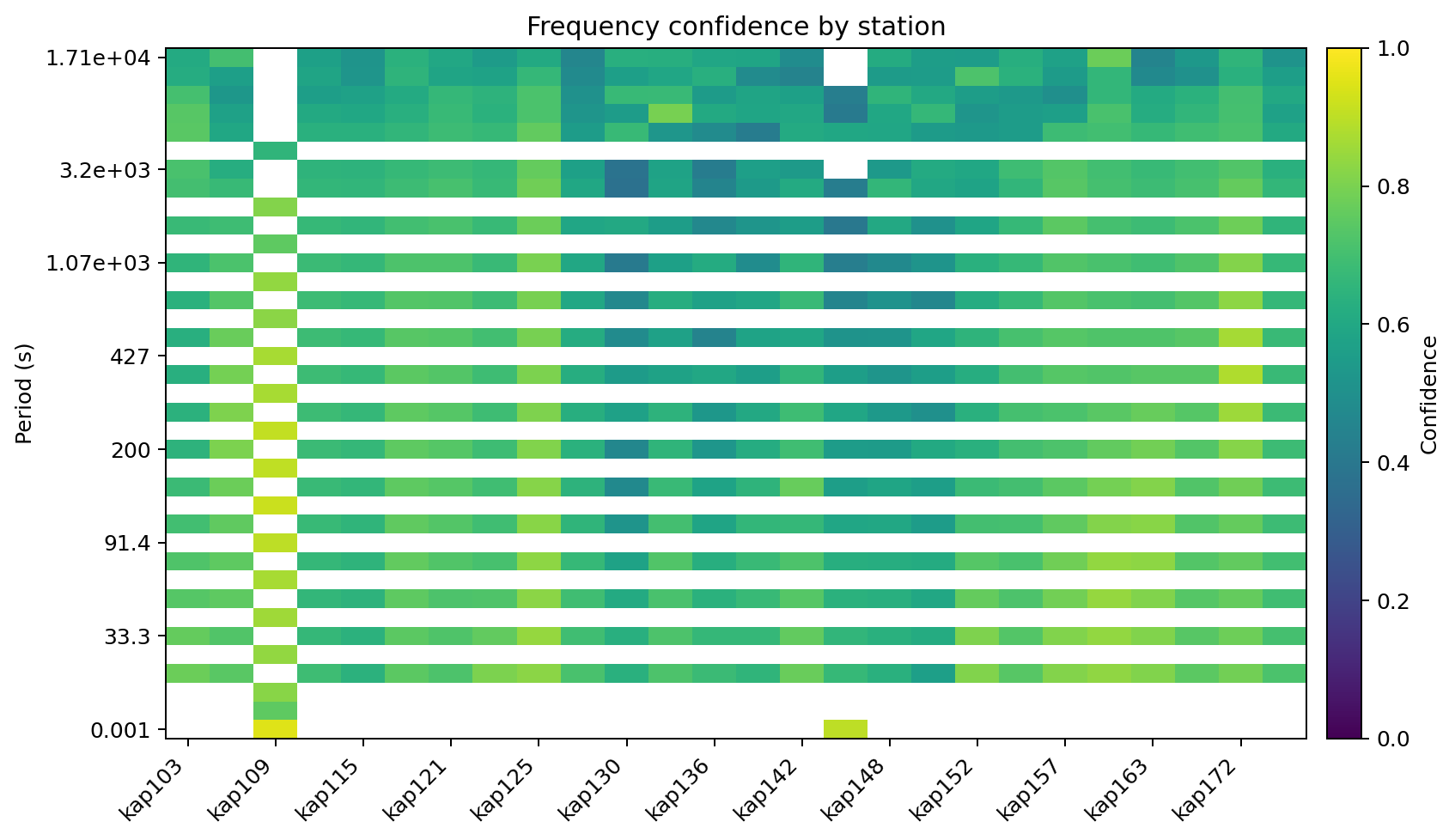
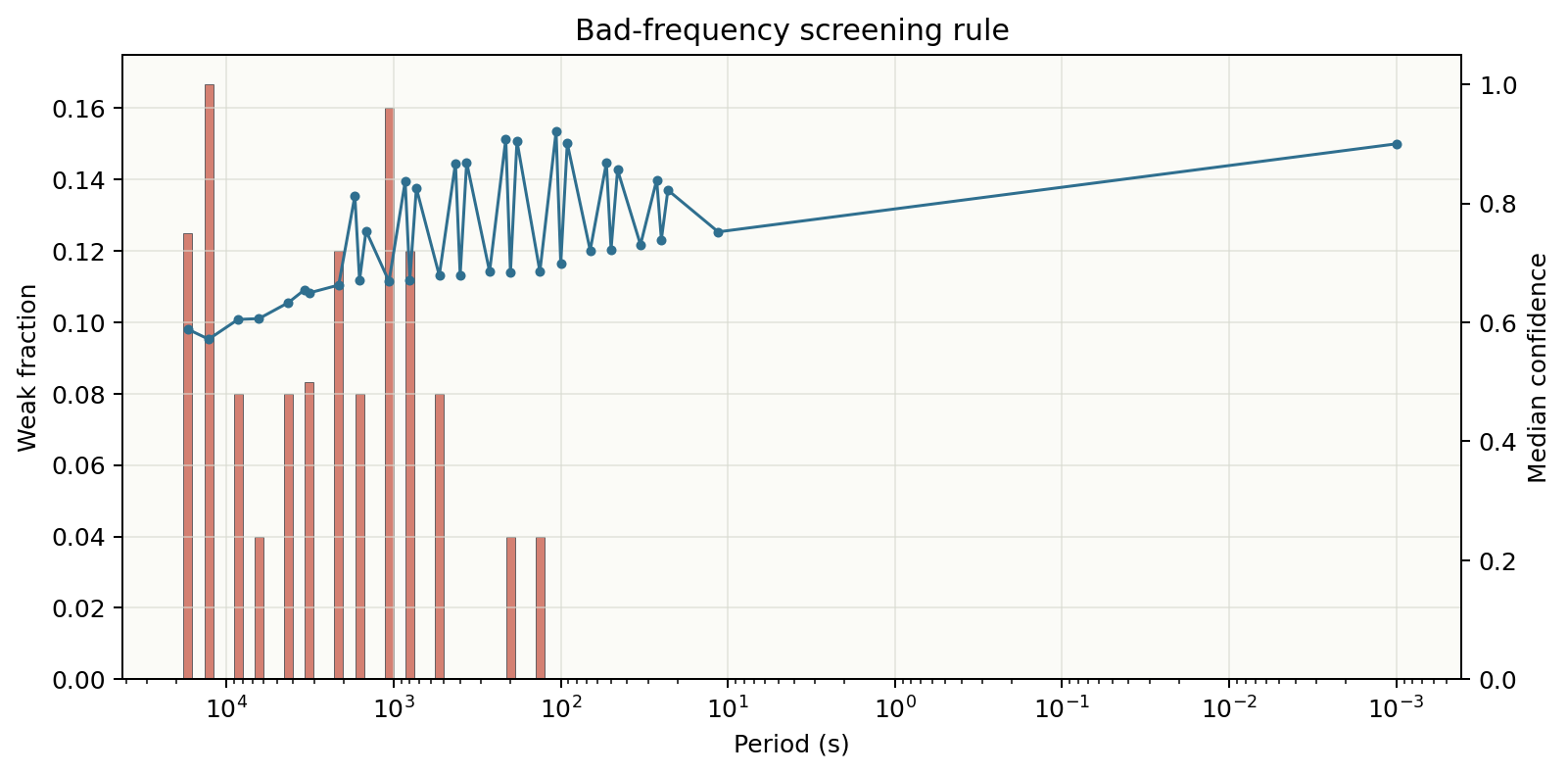
The frequency screen found 518 station-frequency rows and 30 weak rows
(confidence < 0.5), about 5.8 percent of the line.
18.6.7. Drop Weak Rows and Filter Conservatively#
For this data set, the useful operation is row rejection rather than recovery. The measured range ends at 0.04 Hz, so a 50/60 Hz power-line notch cannot act on any sample and is intentionally omitted. Interpolation and polynomial smoothing are also omitted: they would manufacture inversion input. The composite confidence rule drops 30 of 518 station-frequency rows (5.8%) from the impedance tensor and tipper together. A survey-support check then rejects two duplicate 999 Hz rows found only at KAP109; they are incompatible with the common long-period band. Finally, a two-neighbour Hampel filter repairs only isolated magnitude/phase outliers.
>>> conditioned = _processing_chain(functions, sites)
>>> sum(len(s.Z.freq) for s in sites), sum(len(s.Z.freq) for s in conditioned)
(518, 486)
View the executed frequency rejection and Hampel filtering codeClick to inspect and copy the complete code
 1def _processing_chain(functions, sites):
 2    """Drop demonstrably weak rows, then repair only isolated spikes."""
 3    with warnings.catch_warnings():
 4        warnings.filterwarnings("ignore", message="All-NaN slice encountered")
 5        dropped = functions["drop_low_confidence_frequencies"](
 6            sites,
 7            method="composite",
 8            threshold=0.5,
 9            also="both",
10            recursive=False,
11        )
12        supported = functions["drop_freqs_manual"](
13            dropped, drop_freqs=(999.0,), tol_rel=0.005,
14            inplace=False, recursive=False,
15        )
16        filtered = functions["hampel_filter_freq"](
17            supported,
18            win=2,
19            nsig=3.0,
20            on="both",
21            domain="magphase",
22            recursive=False,
23        )
24    return filtered
This pseudosection is produced by
plot_frequency_confidence_psection(); the edit panel
below is produced by plot_frequency_edit_decisions().
Consequently the displayed decisions use the same confidence implementation
as drop_low_confidence_frequencies rather than a separately coded mask.
>>> from pycsamt.emtools import plot_frequency_edit_decisions
>>> ax = plot_frequency_edit_decisions(
...     sites, conditioned, method="composite", ci_hi=0.9, ci_lo=0.5,
...     station_label_step=2,
... )
>>> ax.get_title()
'Frequency edit decisions'
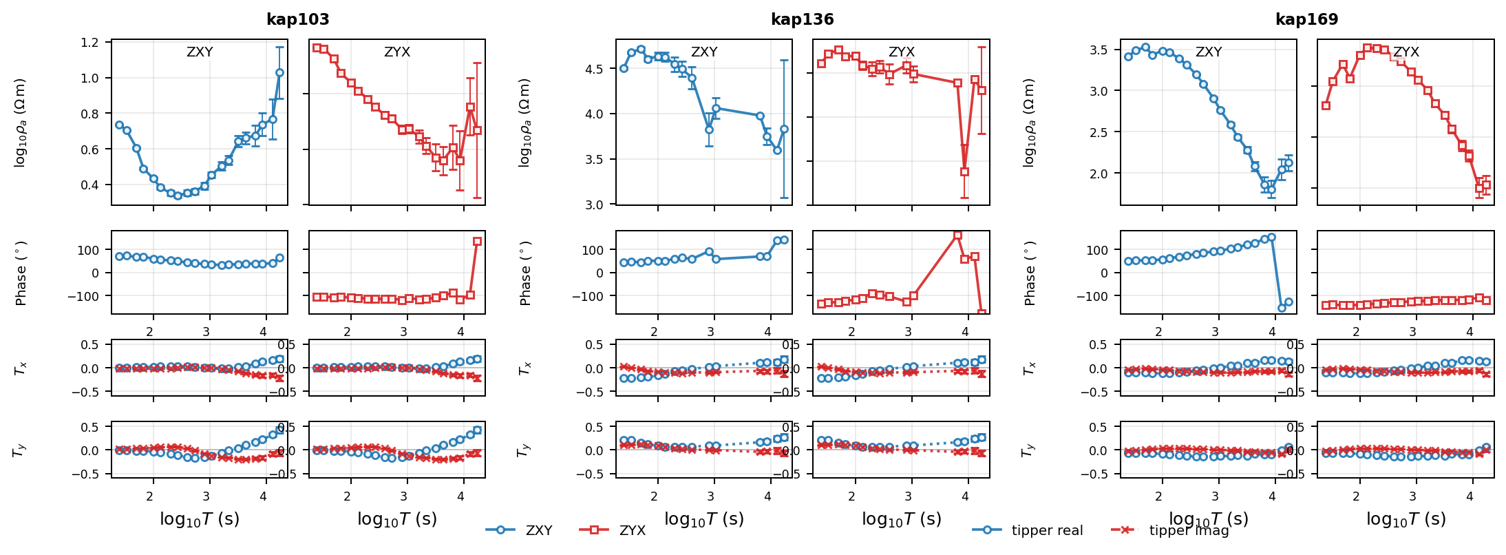
The next matched figures use plot_response_tipper twice, first on the raw
collection and then on the conditioned, rotated collection. KAP103 samples the
southwest, KAP136 the documented cultural-noise corridor, and KAP169 the
northeast. Keeping the panels separate preserves the package’s error bars and
avoids obscuring rejected samples with an overlay.
View the executed three-station comparison codeClick to inspect and copy the complete code
 1def _plot_three_station_raw_corrected(raw_sites, corrected_sites) -> None:
 2    """Use the public response API for matched raw and corrected panels."""
 3    from pycsamt.emtools import plot_response_tipper
 4
 5    stations = ["kap103", "kap136", "kap169"]
 6    for data, raw, filename in (
 7        (raw_sites, True, "kp_three_station_raw.png"),
 8        (corrected_sites, False, "kp_three_station_corrected.png"),
 9    ):
10        fig = plot_response_tipper(
11            data, stations=stations, components=("xy", "yx"), raw=raw,
12            ncols_groups=3, show_error_bars=True,
13            show_tipper_error_bars=True, recursive=False,
14        )
15        _save(fig, filename)
18.6.8. Check Dimensionality and Induction Vectors#
Frequency confidence says whether a row is usable; it does not establish that the Earth is 2-D. The public dimensionality and ellipticity pseudosections add that geological test after conditioning and before selecting a rotation:
>>> from pycsamt.emtools import (
...     plot_dimensionality_psection,
...     plot_ellipticity_psection,
... )
>>> dim_ax = plot_dimensionality_psection(
...     conditioned, skew_th=3.0, ellipt_th=0.2, recursive=False,
... )
>>> ell_ax = plot_ellipticity_psection(
...     conditioned, agg="median", recursive=False,
... )
>>> dim_ax.get_ylabel(), ell_ax.get_ylabel()
('$\\log_{10}(T)$ (s)', '$\\log_{10}(T)$ (s)')
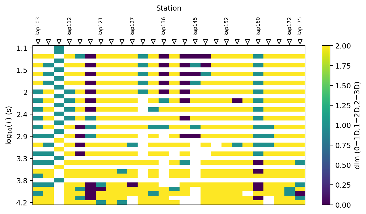
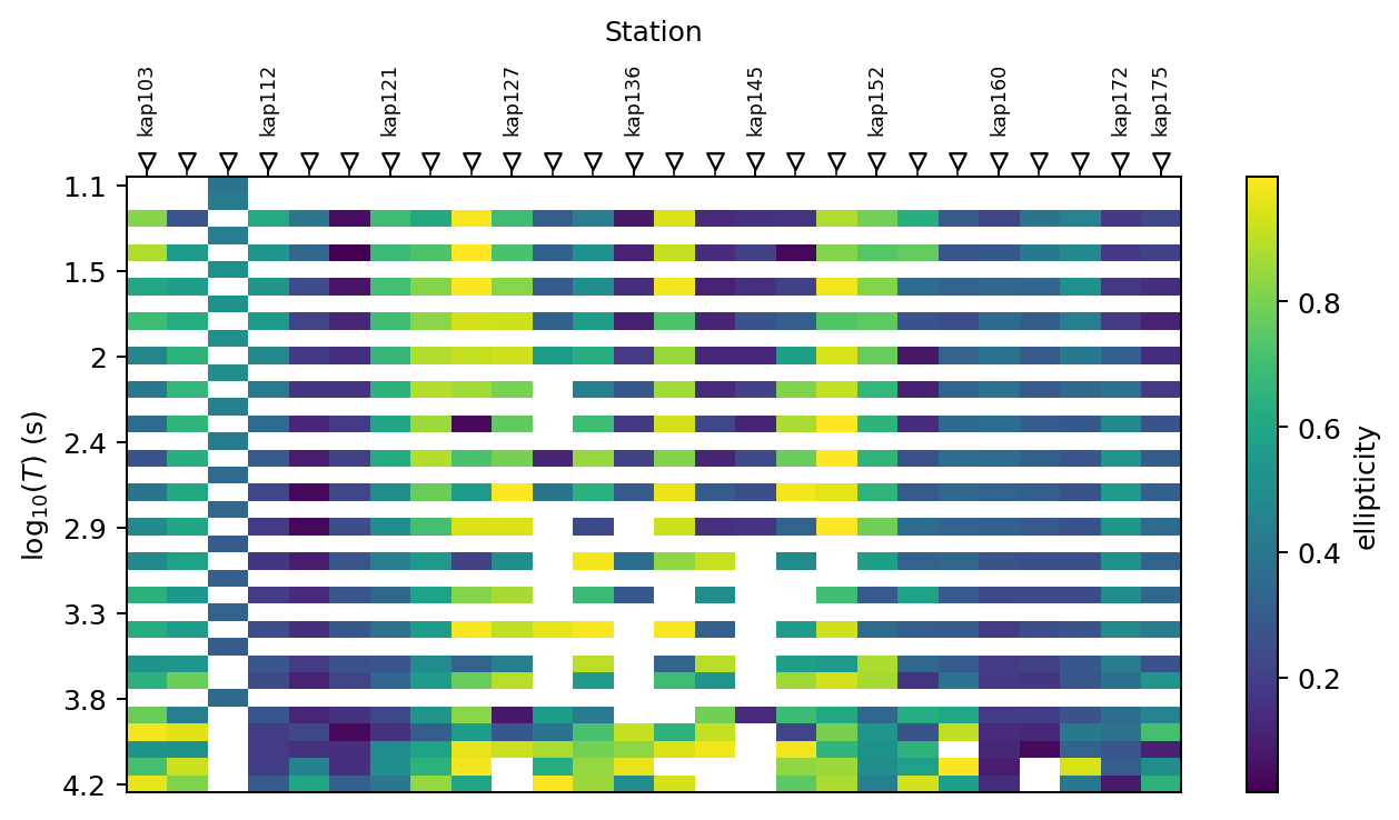
Class 2 (3-D) cells prevail across broad period ranges, and ellipticity varies strongly along the line. This argues against reducing the survey to a uniform 2-D TE/TM problem. White cells are missing or rejected observations, not a fourth dimensionality class.
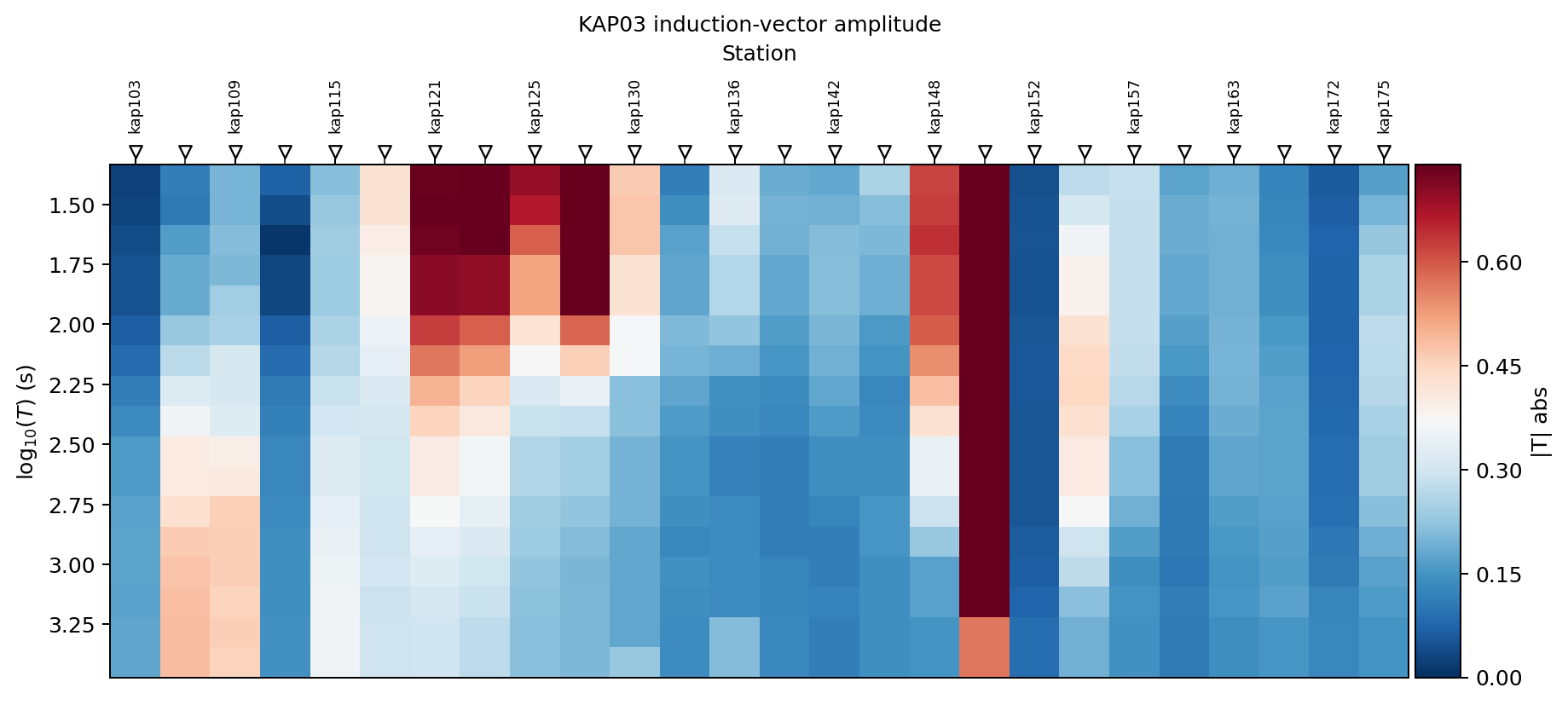
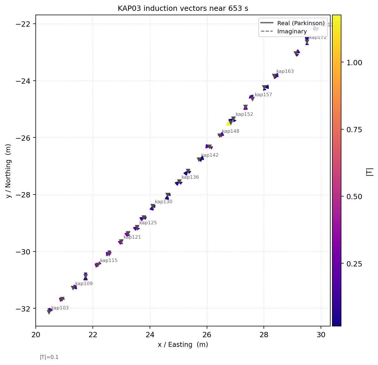
Tipper amplitude and direction provide an independent view of lateral current deflection. The section locates strong responses in station–period space; the map shows their directions near 653.2 s using the Parkinson convention.
>>> from pycsamt.emtools import plot_induction_map, plot_induction_section
>>> section_ax = plot_induction_section(
...     conditioned, component="abs", n_periods=18, recursive=False,
... )
>>> map_ax = plot_induction_map(
...     conditioned, period=653.2, convention="park",
...     show_real=True, show_imag=True, station_labels=True,
...     recursive=False,
... )
>>> len(map_ax.patches) > 0
True
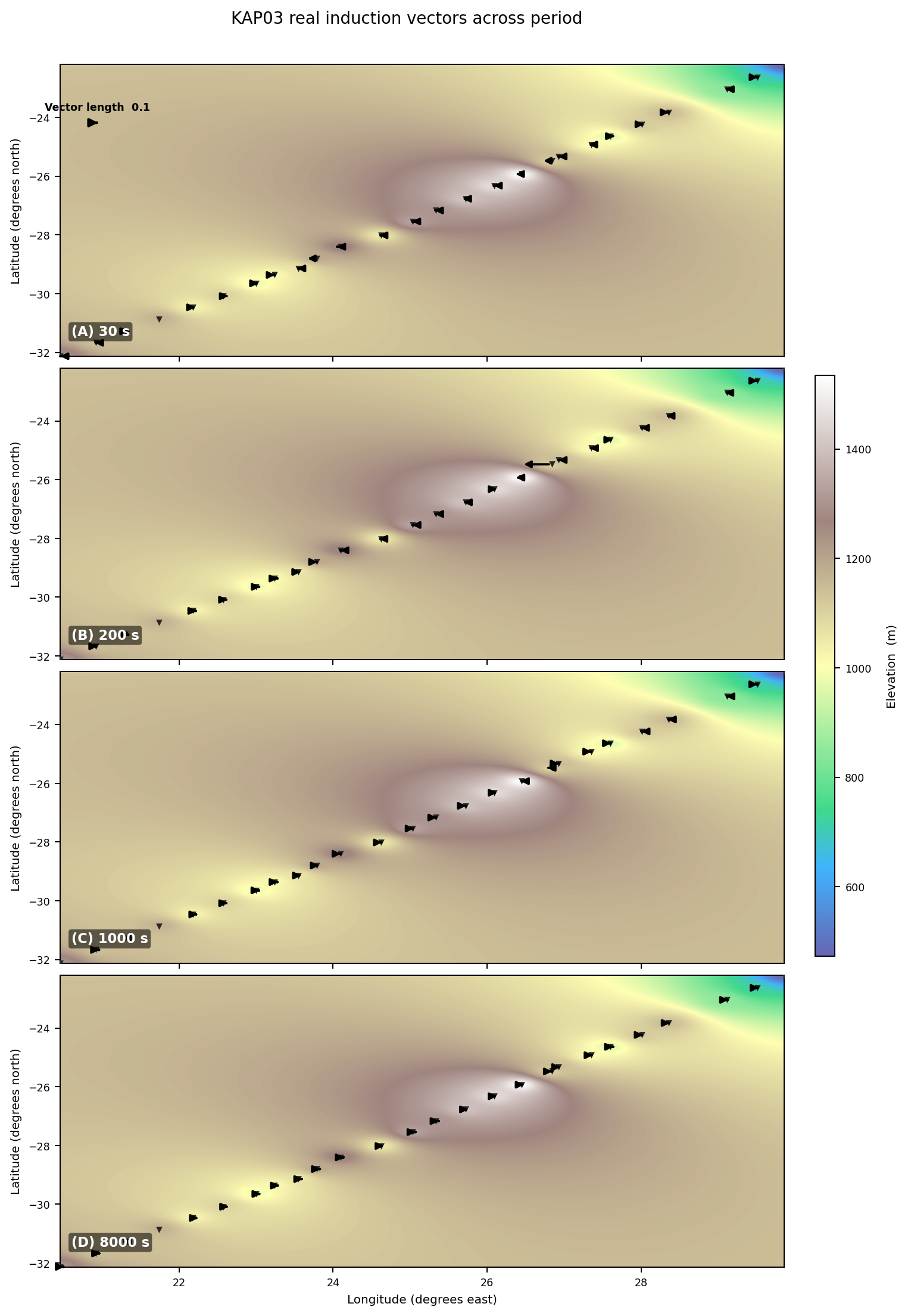
A single target period can conceal reversals or rotations of the induction vector. The multi-period API repeats the real Parkinson arrows over the station-derived topographic surface at four representative penetration scales:
>>> from pycsamt.emtools import plot_induction_multiperiod_map
>>> fig, axes = plot_induction_multiperiod_map(
...     conditioned, periods=(30.0, 200.0, 1000.0, 8000.0),
...     convention="park", background=dem,
...     background_extent=extent, background_cmap="terrain",
...     xlabel="Longitude (degrees east)",
...     ylabel="Latitude (degrees north)",
...     recursive=False,
... )
>>> len(axes)
4
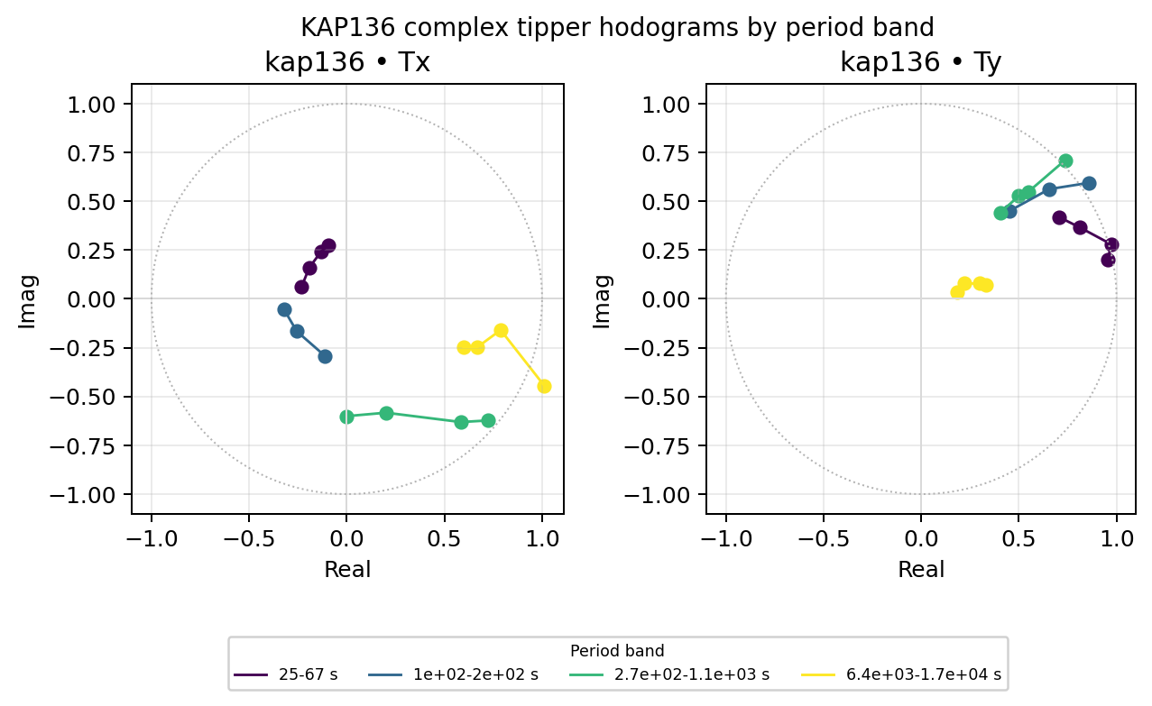
The same transfer function can be inspected in the complex plane. A tipper
hodogram plots real against imaginary response separately for \(T_x\) and
\(T_y\); curvature, clustering, and changes between period bands expose
frequency-dependent induction behavior that a magnitude section alone can
hide. Here normalize=True expands the small measured response relative to
the reference circle for shape comparison; use False when absolute tipper
magnitude must remain visible.
>>> from pycsamt.emtools import plot_tipper_hodograms
>>> fig = plot_tipper_hodograms(
...     conditioned, station="kap136", n_bands=4,
...     normalize=True, ms=2.5, lw=1.15,
...     unit_circle=True, recursive=False,
... )
>>> [ax.get_title() for ax in fig.axes]
['kap136 • Tx', 'kap136 • Ty']
The amplitude section highlights strong lateral responses around KAP121–130, KAP148, and KAP157 over different period bands. Coherent map arrows confirm that the vertical magnetic response carries directional information. Under the adopted convention, Parkinson arrows point toward conductive anomalies; they must be interpreted with phase tensors and topography rather than used as stand-alone strike estimates.
View the dimensionality and induction-vector plotting codeClick to inspect and copy the complete code
 1def _plot_dimensionality_and_induction(functions, sites) -> None:
 2    """Use public dimensionality and induction-vector diagnostics."""
 3    ax = functions["plot_dimensionality_psection"](
 4        sites, skew_th=3.0, ellipt_th=0.2, recursive=False
 5    )
 6    _save(ax.figure, "kp_dimensionality_psection.png")
 7
 8    ax = functions["plot_ellipticity_psection"](
 9        sites, agg="median", recursive=False
10    )
11    _save(ax.figure, "kp_ellipticity_psection.png")
12
13    ax = functions["plot_induction_section"](
14        sites, component="abs", n_periods=18,
15        title="KAP03 induction-vector amplitude", recursive=False,
16    )
17    _save(ax.figure, "kp_induction_section.png")
18
19    ax = functions["plot_induction_map"](
20        sites, period=653.2, convention="park", show_real=True,
21        show_imag=True, station_labels=True,
22        title="KAP03 induction vectors near 653 s", recursive=False,
23    )
24    _save(ax.figure, "kp_induction_map_653s.png")
25
26    topo = pd.read_csv(TOPO_CSV)
27    gx = np.linspace(topo.longitude.min(), topo.longitude.max(), 180)
28    gy = np.linspace(topo.latitude.min(), topo.latitude.max(), 140)
29    xx, yy = np.meshgrid(gx, gy)
30    dx = xx[..., None] - topo.longitude.to_numpy()[None, None, :]
31    dy = yy[..., None] - topo.latitude.to_numpy()[None, None, :]
32    weights = 1.0 / np.maximum(dx * dx + dy * dy, 1e-10)
33    dem = np.sum(weights * topo.elevation_m.to_numpy(), axis=2) / np.sum(weights, axis=2)
34    extent = (gx.min(), gx.max(), gy.min(), gy.max())
35    fig, _ = functions["plot_induction_multiperiod_map"](
36        sites, periods=(30.0, 200.0, 1000.0, 8000.0),
37        convention="park", background=dem, background_extent=extent,
38        background_cmap="terrain", background_clim=(topo.elevation_m.min(), topo.elevation_m.max()),
39        station_labels=False, title="KAP03 real induction vectors across period",
40        xlabel="Longitude (degrees east)", ylabel="Latitude (degrees north)",
41        recursive=False,
42    )
43    _save(fig, "kp_induction_multiperiod_map.png")
44
45    fig = functions["plot_tipper_hodograms"](
46        sites, station="kap136", n_bands=4, normalize=True,
47        ms=2.5, lw=1.15, unit_circle=True, figsize=(8.2, 4.2), recursive=False,
48    )
49    fig.suptitle("KAP136 complex tipper hodograms by period band", fontsize=11)
50    _save(fig, "kp_tipper_hodograms_kap136.png")
18.6.9. Test, Then Reject, Automatic Static Shift#
The static shift diagnostic estimates a frequency-independent impedance factor. It changes apparent-resistivity scale but not phase. Here we calculate a trial only; it is not passed to strike analysis, rotation, or export.
>>> factors, shifted_trial = _static_shift(functions, sites, sites)
>>> factors[["station", "fac_z"]].head(6).round(3).to_dict("records")
[{'station': 'kap103', 'fac_z': 1.91}, {'station': 'kap106', 'fac_z': 1.61}, {'station': 'kap109', 'fac_z': 0.529}, {'station': 'kap112', 'fac_z': 0.237}, {'station': 'kap115', 'fac_z': 3.17}, {'station': 'kap118', 'fac_z': 0.289}]
station  fac_z  fac_z_reviewed  n_used
 kap103   1.91            1.91      20
 kap106   1.61            1.61      20
 kap109  0.529           0.529      18
 kap112  0.237            0.35      20
 kap115   3.17            2.85      20
 kap118  0.289            0.35      20
 kap121  0.578           0.578      20
 kap123   1.35            1.35      20
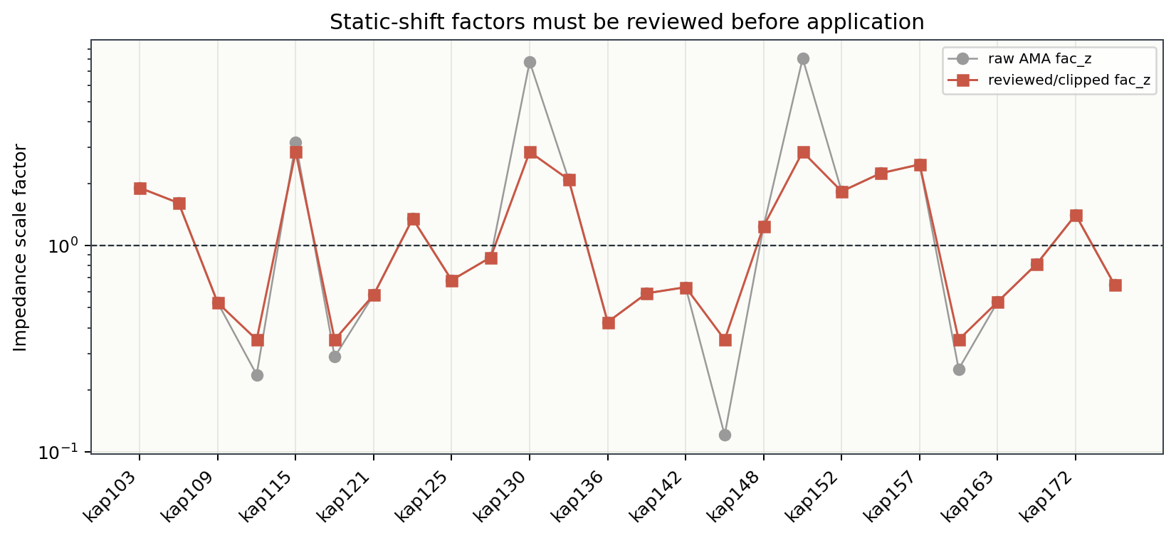
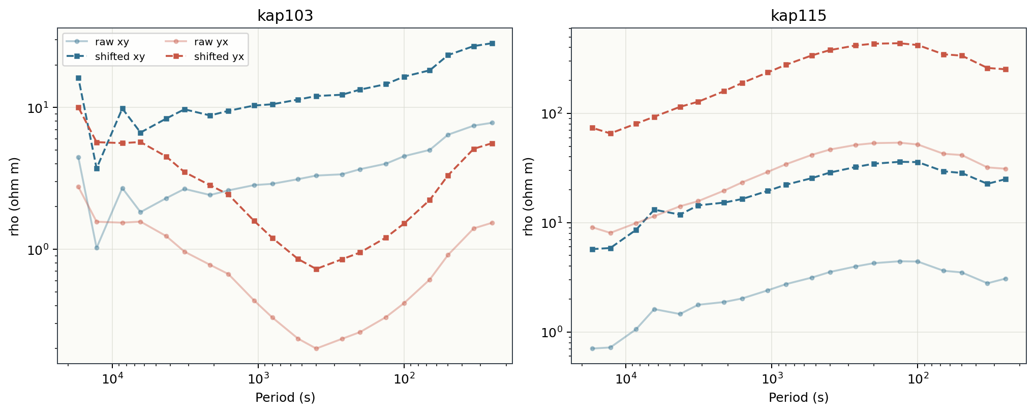
Factors from 0.237 to 3.17 in only the first six sites imply large amplitude
changes. With approximately 60 km station spacing, strong 3-D structure, and
known cultural contamination, neighbour-based amplitude leveling is not
sufficiently constrained. Clipping those values would conceal the diagnostic
failure. We therefore reject the trial and keep conditioned downstream.
Static shift can be revisited with independent near-surface constraints or a
justified distortion model.
View the diagnostic static-shift trial codeClick to inspect and copy the complete code
 1def _static_shift(functions, estimate_sites, apply_sites):
 2    factors = functions["estimate_ss_ama"](
 3        estimate_sites,
 4        sort_by="name",
 5        half_window=3,
 6        max_skew=None,
 7        recursive=False,
 8        api=True,
 9    ).to_pandas(copy=True)
10    factors["fac_z_reviewed"] = factors["fac_z"].clip(lower=0.35, upper=2.85)
11    applied = factors[["station", "fac_z_reviewed"]].rename(
12        columns={"fac_z_reviewed": "fac_z"}
13    )
14    shifted = functions["apply_ss_factors"](
15        apply_sites,
16        applied,
17        key="fac_z",
18        inplace=False,
19        recursive=False,
20    )
21    return factors, shifted
18.6.10. Estimate Strike and Plot Phase Tensors#
After QC and rejection of the static-shift trial, estimate a dominant
geoelectric strike direction from conditioned. The public
estimate_strike_consensus API combines the impedance sweep and
phase-tensor estimates. We then use an inverse-IQR-weighted axial mean and map
the 180-degree-equivalent result into the signed rotation interval:
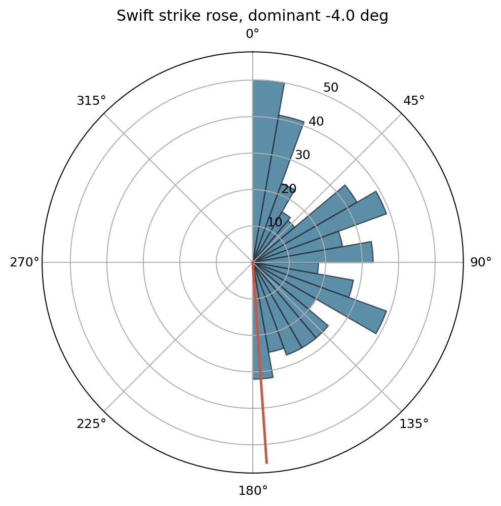
>>> dominant, strike_detail = _dominant_strike(functions, conditioned)
>>> print(f"dominant_strike_deg={dominant:.2f}")
dominant_strike_deg=-39.69
The equivalent axial direction is 140.31 degrees. The broad rose remains evidence of period-dependent or 3-D behaviour, so -39.69 degrees is a pragmatic common frame rather than proof that the whole profile is 2-D.
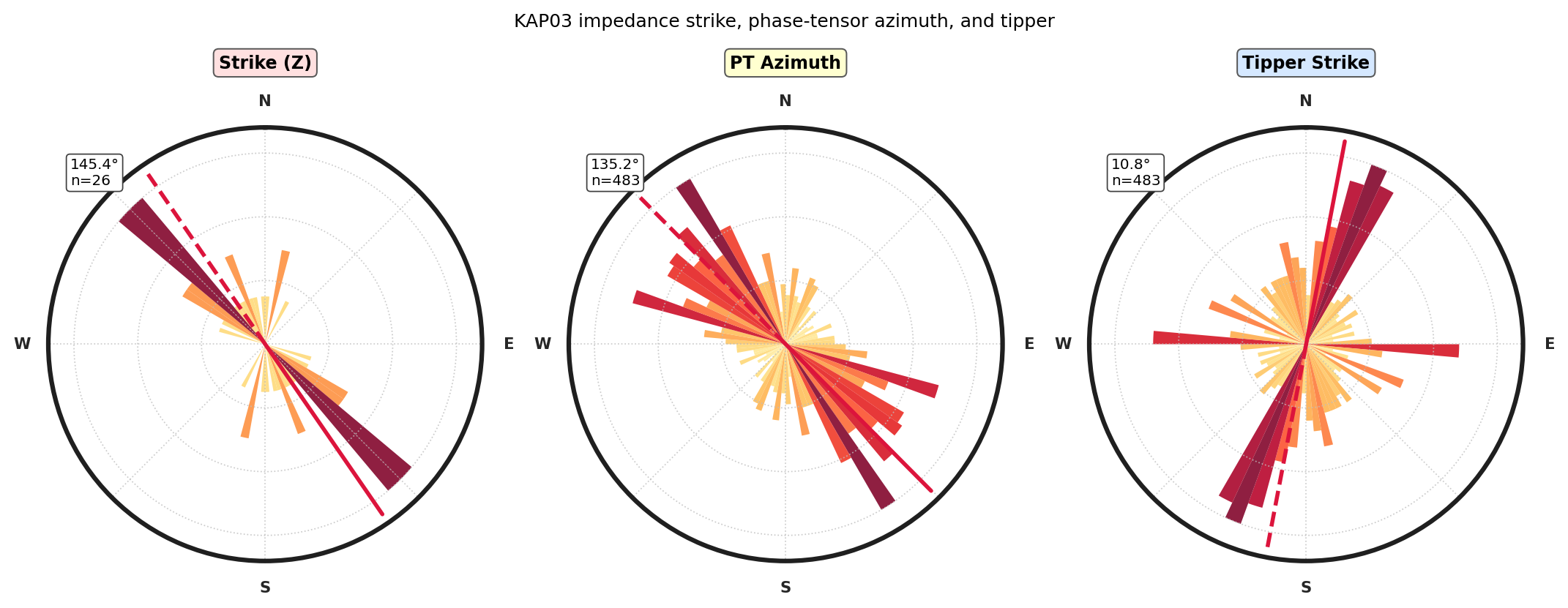
>>> from pycsamt.emtools import plot_strike_analysis, plot_strike_rose
>>> rose = plot_strike_rose(conditioned, method="consensus", recursive=False)
>>> comparison = plot_strike_analysis(
...     conditioned, method="consensus", recursive=False,
... )
>>> len(comparison.axes)
3
The package comparison is especially useful here: impedance and phase-tensor azimuth occupy similar northwest–southeast axial quadrants, whereas the real tipper direction clusters nearer north–south. That disagreement supports retaining full-tensor plus tipper data for 3-D inversion instead of claiming a clean two-dimensional TE/TM decomposition.
View the axial circular-mean strike calculationClick to inspect and copy the complete code
 1def _dominant_strike(functions, sites) -> tuple[float, pd.DataFrame]:
 2    detail = functions["estimate_strike_consensus"](sites, recursive=False)
 3    angles = detail["ang"].to_numpy(dtype=float)
 4    weights = 1.0 / np.maximum(detail["iqr"].to_numpy(dtype=float), 1e-6)
 5    doubled = np.deg2rad(2.0 * angles)
 6    axial = 0.5 * np.rad2deg(
 7        np.arctan2(np.sum(weights * np.sin(doubled)),
 8                   np.sum(weights * np.cos(doubled)))
 9    ) % 180.0
10    signed = ((axial + 90.0) % 180.0) - 90.0
11    return float(signed), detail
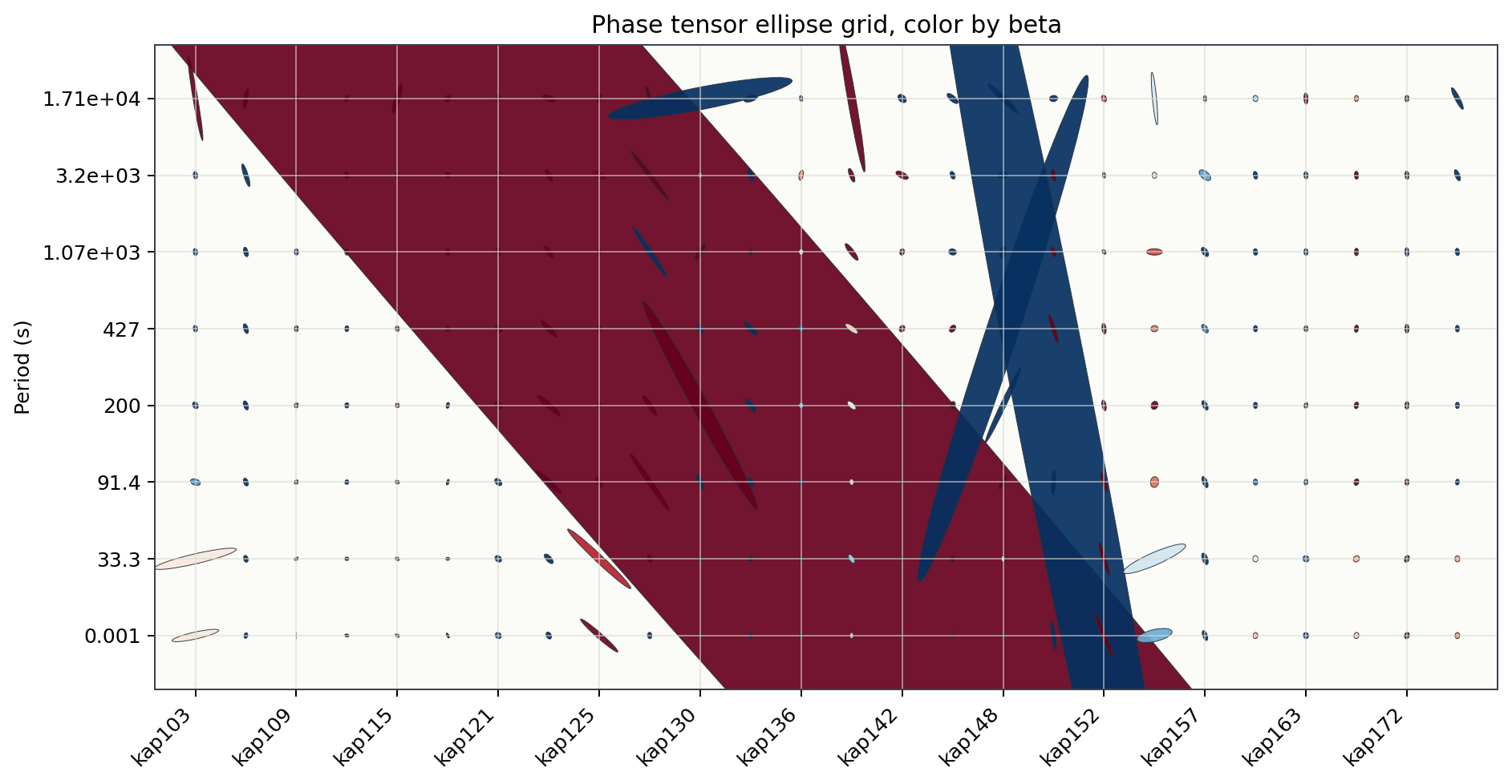
Phase tensor ellipses show orientation, ellipticity, and skew-like behavior without relying on static-shift-sensitive amplitudes:
>>> pt = _plot_phase_tensor_grid(functions, conditioned)
>>> len(pt), pt.station.nunique()
(483, 26)
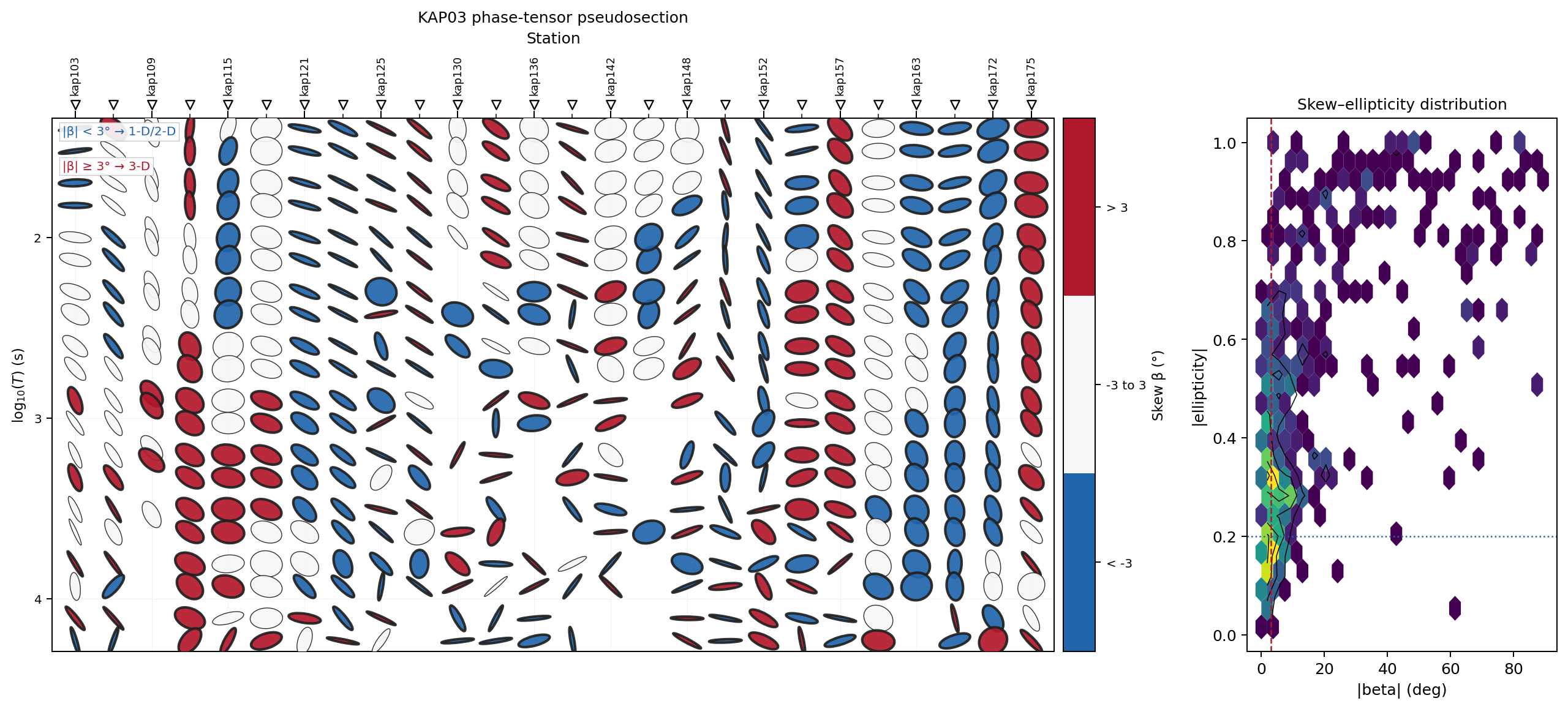
>>> from pycsamt.emtools import plot_phase_tensor_psection
>>> ax = plot_phase_tensor_psection(
...     conditioned, axis_y="logperiod", period_up=False,
...     c_by="beta", normalise_by="shape", min_aspect=0.12,
...     clim=(-3.0, 3.0), color_mode="segmented",
...     ellipse_kws={"edgecolor": "#202020", "linewidth": 0.55},
...     cb_kws={"size": "3.2%", "pad": 0.08}, recursive=False,
... )
>>> ax.get_title()
''
The first grid is retained as the compact tutorial-specific colour-by-data
view. The second is the reusable
plot_phase_tensor_psection() output, with short periods
(high frequencies and shallower sensitivity) at the top. Its visible frame
uses robust finite-data percentiles. Following the common MTpy presentation,
normalise_by="shape" gives every ellipse the same displayed major-axis
length and uses \(|\phi_{\min}/\phi_{\max}|\) for its aspect ratio. The
min_aspect floor prevents unstable near-zero minor axes from becoming
invisible lines; it is a display safeguard and does not alter the tensor.
The segmented colour scale assigns one colour below \(-3^\circ\), a
neutral colour from \(-3^\circ\) to \(+3^\circ\), and one colour above
\(+3^\circ\). This is the compact MTpy-style dimensionality view. Set
color_mode="continuous" to recover a continuous gradient, and customize
the class boundaries and colours with segment_bounds and
segment_colors. The scale is deliberately saturated at \(\beta=\pm3^\circ\), a
widely used dimensionality threshold. Values beyond that interval remain
unchanged in pt and are mapped to the end colours; the plot is therefore a
classification view, not evidence that the raw beta values were clipped.
Pass frame_pct=None for the absolute recorded range,
period_range=(T_min, T_max) for an explicit range, or clim=(lo, hi) for
another fixed cross-survey colour comparison. Omit clim when the purpose is
to inspect the full robust beta distribution instead.
The two-column pseudosection is paired with the compact distribution panel in column three. The dashed \(|\beta|=3^\circ\) and dotted ellipticity \(=0.2\) guides show whether the survey is concentrated in the nominally 1-D/2-D region or contains a substantial distorted/3-D population; they do not reject observations.
Representative station strips provide a less crowded check of how ellipse shape and orientation evolve with period:
>>> from pycsamt.emtools import plot_phase_tensor_strip_grid
>>> fig = plot_phase_tensor_strip_grid(
...     conditioned,
...     profiles={"KAP03": ["kap103", "kap121", "kap148", "kap175"]},
...     c_by="beta", clim=(-3.0, 3.0), normalise_by="cell",
...     min_aspect=0.12, recursive=False,
... )
>>> len(fig.axes) >= 4
True
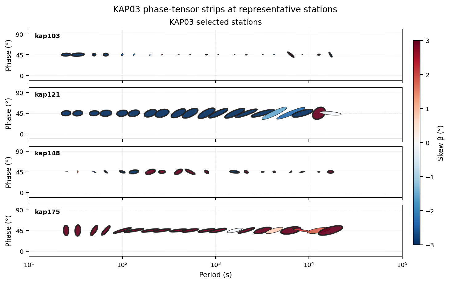
Ellipse orientation changes along the line and across period, while non-zero
beta colours mark departures from an ideal 2-D response. The common
rotation should therefore be accompanied by full-tensor and tipper errors in a
3-D inversion rather than being treated as a guaranteed TE/TM separation.
View the executed phase-tensor ellipse-grid codeClick to inspect and copy the complete code
 1def _plot_phase_tensor_grid(functions, sites) -> pd.DataFrame:
 2    pt = functions["build_phase_tensor_table"](sites, recursive=False)
 3    fig = plt.figure(figsize=(15.0, 6.2))
 4    grid = fig.add_gridspec(1, 3, width_ratios=(1.15, 1.15, 0.8), wspace=0.38)
 5    ax = fig.add_subplot(grid[0, :2])
 6    functions["plot_phase_tensor_psection"](
 7        sites, axis_y="logperiod", period_up=False, c_by="beta",
 8        normalise_by="shape", min_aspect=0.12, clim=(-3.0, 3.0),
 9        color_mode="segmented",
10        ellipse_kws={"edgecolor": "#202020", "linewidth": 0.55},
11        cb_kws={"size": "3.2%", "pad": 0.08, "ticksize": 8},
12        title="KAP03 phase-tensor pseudosection", recursive=False, ax=ax,
13    )
14    density_ax = fig.add_subplot(grid[0, 2])
15    functions["plot_skew_ellipt_density"](
16        sites, gridsize=24, recursive=False, ax=density_ax,
17    )
18    density_ax.axvline(3.0, color="#b2182b", ls="--", lw=1.0)
19    density_ax.axhline(0.2, color="#2166ac", ls=":", lw=1.0)
20    density_ax.set_title("Skew–ellipticity distribution", fontsize=10)
21    fig.subplots_adjust(top=0.90, bottom=0.12, left=0.06, right=0.97)
22    _save(fig, "kp_phase_tensor_psection_api.png")
23
24    strip_fig = functions["plot_phase_tensor_strip_grid"](
25        sites,
26        profiles={"KAP03 selected stations": ["kap103", "kap121", "kap148", "kap175"]},
27        c_by="beta", clim=(-3.0, 3.0), normalise_by="cell",
28        min_aspect=0.12, edgecolor="#202020", linewidth=0.55,
29        suptitle="KAP03 phase-tensor strips at representative stations",
30        panel_size=(8.0, 1.25), recursive=False,
31    )
32    _save(strip_fig, "kp_phase_tensor_strip_grid.png")
33    stations = list(dict.fromkeys(pt["station"]))
34    periods = np.array(sorted(pt["period"].unique()))
35    selected = periods[
36        np.linspace(0, len(periods) - 1, min(8, len(periods))).astype(int)
37    ]
38    fig, ax = plt.subplots(figsize=(12.0, 5.8))
39    max_s1 = np.nanpercentile(pt["s1"], 90)
40    for ix, station in enumerate(stations):
41        sdf = pt[pt["station"] == station]
42        for period in selected:
43            row = sdf.iloc[(sdf["period"] - period).abs().argsort()[:1]]
44            if row.empty:
45                continue
46            r = row.iloc[0]
47            y = np.where(selected == period)[0][0]
48            width = 0.55 * float(r["s1"]) / max(max_s1, 1e-9)
49            height = max(
50                0.08,
51                width * max(float(r["s2"]) / max(float(r["s1"]), 1e-9), 0.08),
52            )
53            ell = Ellipse(
54                (ix, y),
55                width=width,
56                height=height,
57                angle=float(r["theta"]),
58                facecolor=plt.cm.RdBu_r(
59                    np.clip((float(r["beta"]) + 20) / 40, 0, 1)
60                ),
61                edgecolor="#27323a",
62                linewidth=0.4,
63                alpha=0.92,
64            )
65            ax.add_patch(ell)
66    ax.set_xlim(-0.8, len(stations) - 0.2)
67    ax.set_ylim(-0.7, len(selected) - 0.3)
68    ax.set_xticks(np.arange(0, len(stations), 2))
69    ax.set_xticklabels(stations[::2], rotation=45, ha="right")
70    ax.set_yticks(np.arange(len(selected)))
71    ax.set_yticklabels([f"{p:.3g}" for p in selected])
72    ax.invert_yaxis()
73    ax.set_ylabel("Period (s)")
74    ax.set_title("Phase tensor ellipse grid, color by beta")
75    _style_axis(ax)
76    _save(fig, "kp_phase_tensor_grid.png")
77    return pt
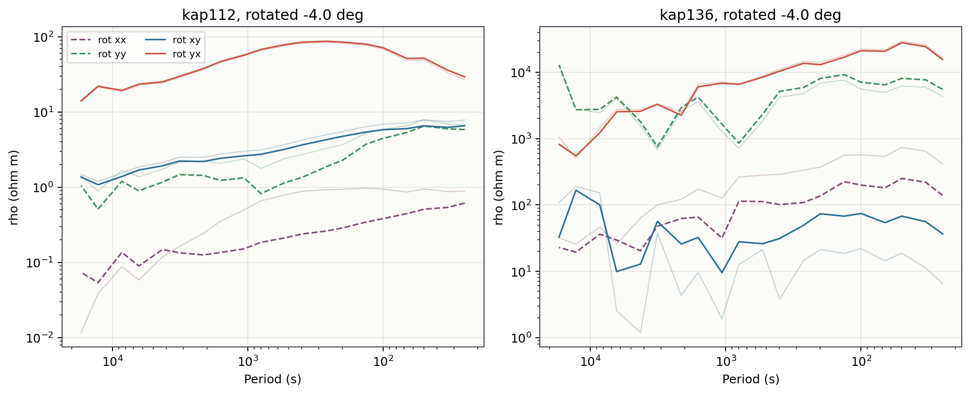
18.6.11. Rotate Impedance and Tipper#
Rotate both impedance and tipper into the selected coordinate frame before exporting inversion-ready EDIs:
>>> rotated = _rotate_sites(conditioned, dominant)
>>> len(rotated), all(getattr(s, "Tip", None) is not None for s in rotated)
(26, True)
The goal of rotation is not to make the data look perfect. It should reduce coordinate-frame mixing and make TE/TM separation more interpretable when the strike estimate is stable enough.
View the impedance-and-tipper rotation codeClick to inspect and copy the complete code
1def _rotate_sites(sites, angle_deg: float):
2    rotated = copy.deepcopy(sites)
3    for site in rotated:
4        ed = _edi(site)
5        ed.Z.rotate(angle_deg)
6        tip = getattr(ed, "Tip", None)
7        if tip is not None:
8            tip.rotate(angle_deg)
9    return rotated
18.6.12. Export and Prove the EDI Round Trip#
Write only the rotated collection: it contains sourced coordinates and
topography, synchronized impedance and tipper rows, the conservative filter,
and the documented -39.69-degree rotation. Reloading the files is part of the
workflow, because a successful write alone does not prove that metadata and
transfer functions survived serialization.
>>> written, checked, elevations = _export_and_validate(functions, rotated)
>>> len(written), len(checked), sum(s.Tip is not None for s in checked)
(26, 26, 26)
>>> float(elevations.min()), float(elevations.max())
(473.0, 1535.0)
The inversion-ready files and their manifest are written to
results/kap03_mt_tutorial/edi_conditioned_rotated. These checked EDIs–not
the raw files or the rejected static-shift trial–are the input for later ModEM
mesh, error-floor, and inversion examples.
View the executed EDI export and round-trip validation codeClick to inspect and copy the complete code
 1def _export_and_validate(functions, sites):
 2    """Write conditioned EDIs and prove coordinates, tipper, and inventory survive."""
 3    from pycsamt.site.export import write_sites
 4
 5    edi_out = RESULT_DIR / "edi_conditioned_rotated"
 6    written = write_sites(
 7        sites, edi_out, exist_ok=True, manifest_csv=edi_out / "manifest.csv"
 8    )
 9    reloaded = functions["ensure_sites"](
10        edi_out, recursive=False, strict=True
11    ).ordered()
12    if len(written) != len(sites) or len(reloaded) != len(sites):
13        raise RuntimeError("conditioned EDI export/reload inventory mismatch")
14    if not all(getattr(_edi(site), "Tip", None) is not None for site in reloaded):
15        raise RuntimeError("tipper was lost during EDI round trip")
16    elevations = np.asarray(
17        [float(_edi(site).get_section("head").elev) for site in reloaded]
18    )
19    return written, reloaded, elevations
18.6.13. Prepare the Classical 3-D ModEM Inversion#
The round-tripped EDIs are now the sole input to the classical branch. ModEM minimizes a regularized objective of the form
where \(\mathbf F\) is the 3-D forward operator, \(\mathbf W_d\) contains inverse data uncertainties, \(\mathbf W_m\) implements model smoothness, and \(\lambda\) controls the fit–roughness trade-off. Consequently, the error floor and covariance file are part of the scientific model, not merely file format settings.
For KAP03 we use all four impedance components, an 8% impedance error floor, six air layers, 28 earth layers, and a 100 \(\Omega\,\mathrm m\) half-space. The 25 km horizontal core scale reflects this unusually long regional transect; copying that value to a compact AMT survey would be a mistake.
>>> from pycsamt.models.modem import InputBuilder, ModEmConfig
>>> cfg = ModEmConfig(
...     mode="3d", component_type="Full_Impedance",
...     error_floor_z=0.08, freq_min=5e-5, freq_max=0.04,
...     cell_size_h=25_000.0, n_padding_xy=5,
...     nz=28, n_airlayers=6, cell_size_v_top=250.0,
...     depth_scale=1.25, initial_rho=100.0,
...     smooth_x=0.3, smooth_y=0.3, smooth_z=0.2,
...     max_iterations=100, target_rms=1.05,
...     use_mpi=True, n_procs=8,
... )
>>> builder = InputBuilder(config=cfg)
>>> files = builder.build(
...     checked, workdir="results/kap03_mt_tutorial/inversion/modem3d",
...     data_filename="KAP03_ModEM.dat",
...     model_filename="KAP03_m0.ws",
...     cov_filename="KAP03.cov", ctrl_filename="KAP03.inv",
... )
>>> sorted(files)
['control', 'covariance', 'data', 'model']
>>> builder.model.shape, builder.model.n_air
((34, 49, 58), 6)
The executed build reaches 515,988 m cumulative earth depth. That is a mesh boundary, not a claim that every cell is resolved. Deep padding reduces boundary influence; sensitivity and resolution must still be assessed from the recovered model and response residuals.
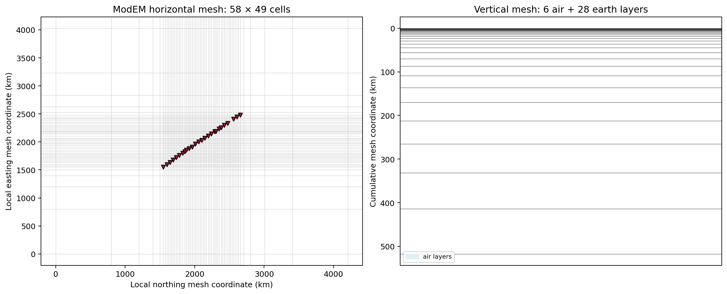
The dense central cells cover the station footprint while geometric padding moves the numerical boundaries away from it. The vertical panel makes the rapid depth growth explicit. The current ModEM builder writes full impedance but not the EDI tipper block, so the conditioned tipper is retained for independent directional QC rather than silently claimed as inverted data.
View the executed ModEM input-builder codeClick to inspect and copy the complete code
 1def build_modem_inputs(sites):
 2    """Write and reload the complete classical ModEM input set."""
 3    from pycsamt.models.modem import InputBuilder, ModEmConfig, ModEmRunner
 4    from pycsamt.models.modem.model3d import ModEmModel3D
 5
 6    cfg = ModEmConfig(
 7        mode="3d",
 8        component_type="Full_Impedance",
 9        error_floor_z=0.08,
10        freq_min=5.0e-5,
11        freq_max=0.04,
12        cell_size_h=25_000.0,
13        n_padding_xy=5,
14        nz=28,
15        n_airlayers=6,
16        cell_size_v_top=250.0,
17        depth_scale=1.25,
18        initial_rho=100.0,
19        smooth_x=0.3,
20        smooth_y=0.3,
21        smooth_z=0.2,
22        n_smooth_iter=2,
23        max_iterations=100,
24        target_rms=1.05,
25        use_mpi=True,
26        n_procs=8,
27    )
28    builder = InputBuilder(config=cfg)
29    files = builder.build(
30        sites,
31        workdir=MODEM_DIR,
32        data_filename="KAP03_ModEM.dat",
33        model_filename="KAP03_m0.ws",
34        cov_filename="KAP03.cov",
35        ctrl_filename="KAP03.inv",
36    )
37    model = ModEmModel3D.read(files["model"])
38    command = ModEmRunner(MODEM_DIR, config=cfg).command(
39        files["model"].name,
40        files["data"].name,
41        files["control"].name,
42        covariance=files["covariance"].name,
43    )
44    manifest = {
45        "stations": len(list(sites)),
46        "model_shape_nz_ny_nx": list(model.shape),
47        "earth_depth_m": float(np.sum(model.z_widths[model.n_air :])),
48        "air_layers": int(model.n_air),
49        "files": {key: value.name for key, value in files.items()},
50        "dry_run_command": command,
51        "tipper_note": "Current ModEM builder writes full impedance; retain EDI tipper for independent QC.",
52    }
53    MODEM_DIR.mkdir(parents=True, exist_ok=True)
54    (MODEM_DIR / "build_manifest.json").write_text(
55        json.dumps(manifest, indent=2), encoding="utf-8"
56    )
57    print(json.dumps(manifest, indent=2))
58    return builder, manifest
18.6.14. Compile and Run ModEM#
pyCSAMT prepares inputs and launches a licensed user-supplied executable; it does not redistribute ModEM. Follow ModEM for compiler, MPI, and executable-placement details, then print the command before starting a potentially long run:
>>> from pycsamt.models.modem import ModEmRunner
>>> runner = ModEmRunner(
...     "results/kap03_mt_tutorial/inversion/modem3d", config=cfg,
... )
>>> runner.command(
...     "KAP03_m0.ws", "KAP03_ModEM.dat", "KAP03.inv",
...     covariance="KAP03.cov",
... )
'mpirun -np 8 Mod3DMT -I NLCG KAP03_m0.ws KAP03_ModEM.dat KAP03.inv KAP03.cov'
After checking MPI allocation and disk space, the corresponding execution is:
>>> result = runner.run(
...     "KAP03_m0.ws",
...     "KAP03_ModEM.dat",
...     "KAP03.inv",
...     covariance="KAP03.cov",
...     timeout=None,
... )
The external inversion is intentionally not launched while building this documentation. Once complete, inspect RMS by iteration, component-wise residuals, boundary cells, covariance sensitivity, and whether topographic air cells match the intended terrain before interpreting conductors. The full result-loading workflow is developed in Prepare A ModEM Inversion and Run Classical Inversions: Occam2D, ModEM, and MARE2DEM.
18.6.15. Build an Optional Triangular Profile Mesh#
A mesh need not be rectilinear, but solver compatibility matters. The following topography-following mesh is a genuine quality triangular mesh with 288 nodes and 495 elements. Both axes are expressed in kilometres; the lower panel enlarges the upper 5 km so the measured 1.06 km elevation range is not flattened by the full 300 km MT domain:
>>> mesh = build_profile_triangle_mesh()
triangle_nodes=288 triangle_elements=495
>>> mesh.n_nodes, mesh.n_triangles
(288, 495)
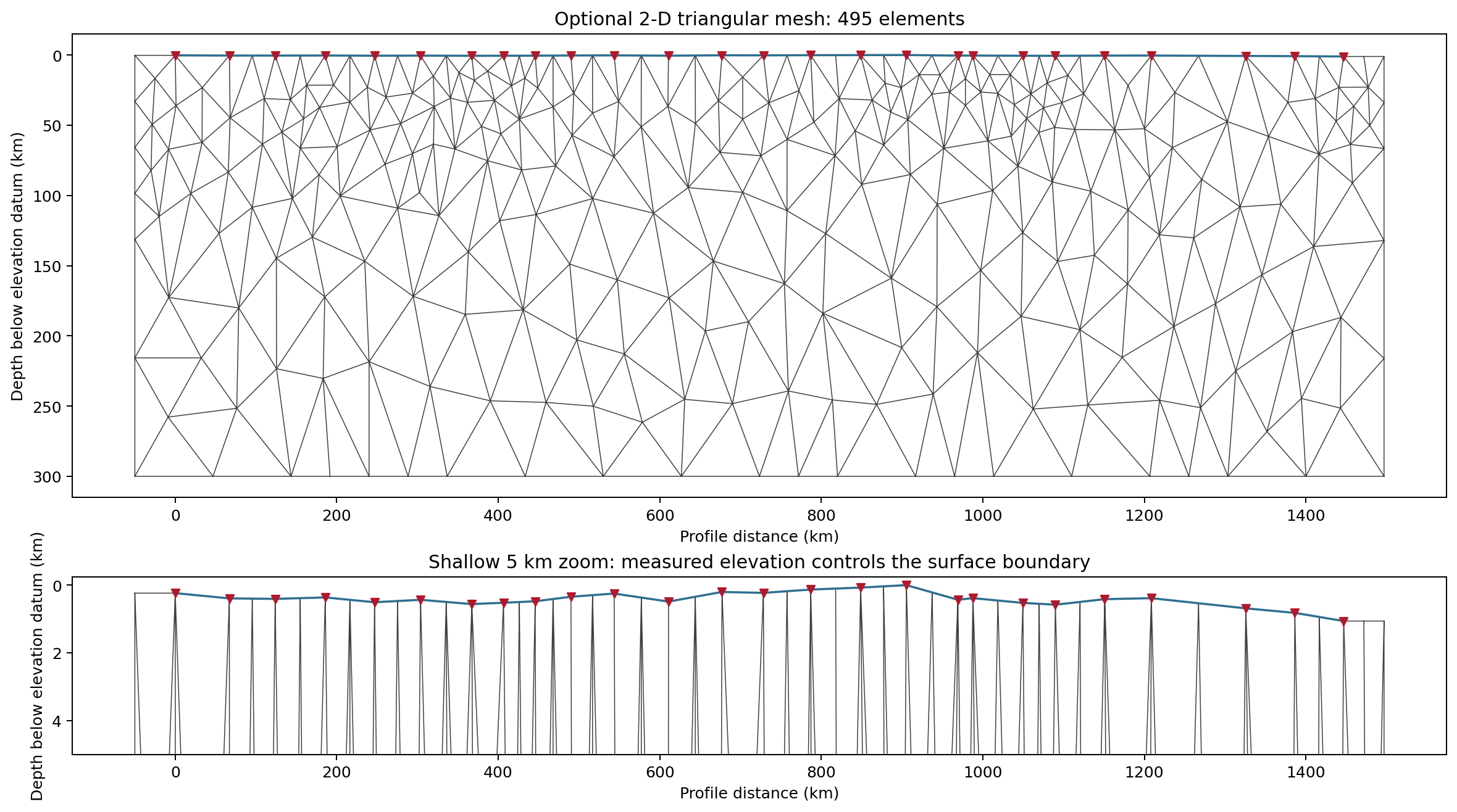
This is an optional 2-D realization for
TriFEM2DAdapter/physics="mt2d_tri". It cannot be passed to ModEM or
MT3DAdapter: both current 3-D engines require a structured mesh. Keeping
that distinction explicit prevents a visually attractive triangulation from
being misreported as the mesh used by a 3-D forward solve.
View the executed topographic triangular-mesh codeClick to inspect and copy the complete code
 1def build_profile_triangle_mesh():
 2    """Build an optional topography-following 2-D triangular realization."""
 3    from pycsamt.api import draw_tri_mesh
 4    from pycsamt.forward.maxwell.tri_mesh_gen import build_graded_tri_mesh
 5
 6    topo = pd.read_csv(TOPO_CSV)
 7    lat = np.deg2rad(topo.latitude.to_numpy())
 8    lon = np.deg2rad(topo.longitude.to_numpy())
 9    seg = 2 * 6_371_008.8 * np.arcsin(np.sqrt(
10        np.sin(np.diff(lat) / 2) ** 2
11        + np.cos(lat[:-1]) * np.cos(lat[1:]) * np.sin(np.diff(lon) / 2) ** 2
12    ))
13    chain = np.r_[0.0, np.cumsum(seg)]
14    surface_depth = topo.elevation_m.max() - topo.elevation_m.to_numpy()
15    pad = 50_000.0
16    mesh = build_graded_tri_mesh(
17        (-pad, float(chain[-1] + pad)),
18        (float(surface_depth.min()), 300_000.0),
19        chain,
20        surface_cell_m=15_000.0,
21        growth_rate=1.35,
22        max_cell_m=80_000.0,
23        min_angle=28.0,
24        topo_x_m=chain,
25        topo_z_m=surface_depth,
26    )
27    from matplotlib.ticker import FuncFormatter
28
29    fig, axes = plt.subplots(
30        2, 1, figsize=(13.0, 7.2), constrained_layout=True,
31        gridspec_kw={"height_ratios": (3.0, 1.15)},
32    )
33    station_z = np.interp(chain, chain, surface_depth)
34    km = FuncFormatter(lambda value, _pos: f"{value / 1000:g}")
35    for ax in axes:
36        draw_tri_mesh(ax, mesh, preset="diagram")
37        ax.plot(chain, surface_depth, color="#2f6f8f", lw=1.4, zorder=4)
38        ax.scatter(chain, station_z, marker="v", color="#b2182b", s=26, zorder=5)
39        ax.xaxis.set_major_formatter(km)
40        ax.yaxis.set_major_formatter(km)
41        ax.set_xlabel("Profile distance (km)")
42        ax.set_ylabel("Depth below elevation datum (km)")
43        ax.invert_yaxis()
44    axes[0].set_title(f"Optional 2-D triangular mesh: {mesh.n_triangles:,} elements")
45    axes[1].set_ylim(5_000.0, -250.0)
46    axes[1].set_title("Shallow 5 km zoom: measured elevation controls the surface boundary")
47    fig.savefig(IMAGE_DIR / "kp_optional_triangular_profile_mesh.png", dpi=180, bbox_inches="tight")
48    plt.close(fig)
49    print(f"triangle_nodes={mesh.n_nodes} triangle_elements={mesh.n_triangles}")
50    return mesh
18.6.16. Configure the MT3D AI Inversion#
The AI branch uses the same corrected EDIs and real station geometry, but its
training pairs come from genuine small-grid 3-D Maxwell simulations through
physics="mt3d". For realization \(i\), the network receives synthetic
responses \(\mathbf x^{(i)}\) and learns the known gridded
log-resistivity \(\mathbf y^{(i)}\) by minimizing
where \(\mathbf A\) is the station adjacency graph. The field prediction is an inference from this synthetic distribution; it is not a replacement for the ModEM objective above and it has no field ground-truth resistivity.
The comparison uses two independent branches. physics="mt2d_tri" learns
on a topography-following triangular mesh, whereas physics="mt3d" learns
on a structured 3-D mesh. Each requests 100 epochs, enables early
stopping with patience 15, uses 200 geological realizations and eight
frequencies inside the measured band. Both meshes stop at 100 km depth
rather than 250 km – KAP03’s own 5e-5-0.04 Hz band does not resolve
structure near 250 km with useful confidence in the first place – but,
unlike an earlier coarsened pass at this same 200-realization count, the
cell sizes below are now deliberately fine rather than coarsened for
speed: MT2D’s mesh_target_cell_m matches the standalone triangular
mesh already shown above, and MT3D’s n_layers doubles the vertical
resolution of the plotted section, the two knobs that actually determine
how blocky each branch’s own figure looks. The MT2D configuration is
concise:
>>> from pycsamt.agents import Inv2DAgent
>>> from pycsamt.forward.maxwell.tri_fem2d import TriFEM2DAdapter
>>> chainage_m, surface_depth_m = profile_geometry()
>>> profile_length_m = chainage_m[-1]
>>> mt2d = Inv2DAgent(
...     physics="mt2d_tri", depth_max=100_000.0,
...     n_train_profiles=200, epochs=100, patience=15,
...     n_freqs=8, n_stations_per_profile=26,
...     station_spacing_m=profile_length_m / 25,
...     mesh_target_cell_m=15_000.0,
...     field_grid_cell_m=7_500.0,
...     gcn_adjacency_radius_m=30_000.0,
...     topo_x_m=chainage_m, topo_z_m=surface_depth_m,
...     mare2dem_adapter=TriFEM2DAdapter(),
... )
The measured elevations therefore enter the MT2D forward mesh, and
mesh_target_cell_m=15,000 now matches the standalone triangular mesh
built earlier rather than the coarser 45,000 m used in an earlier pass at
this tutorial – the triangles actually driving GCN training are no bigger
than the ones already shown in the “optional” mesh figure.
A finer mesh alone made an existing problem visible rather than fixing anything: the first render of this refined mesh showed near-constant resistivity in a “curtain” under each station, unrelated to depth. Two separate things turned out to be going on:
The raw triangle shapes are not actually elongated – measuring them directly gave a median width of 19.7 km against a median height of 19.8 km (ratio 0.99), i.e. genuinely close to isotropic. The vertical “stretch” is a rendering artifact: 100 km of depth is drawn across roughly the same plot width as 1,500 km of profile, so any real triangle looks tall and thin on screen.
The GCN, however, really was depth-blind.
Inv2DAgent’sgcn_adjacency_radius_mhad never been set in any earlier pass of this tutorial, leaving the library default of 300 m in effect on a mesh whose actual median distance between neighbouring triangle centroids is about 10 km – 2-3 orders of magnitude coarser than that radius. Directly rebuilding the adjacency matrix at 300 m on this mesh’s real triangle centroids gives zero edges among all 434,940 possible triangle pairs; after the mandatory self-loops, the “graph” is exactly the identity matrix, so no message-passing was happening at all. Combined with every triangle’s input being only its nearest station’s frequency-sounding curve (no depth or position information), every triangle nearest a given station received an identical input and no cross-triangle mixing, so the network could only predict one value per station regardless of depth – exactly the flat curtain.
Fixing this needed two changes, both now in pycsamt/agents/inv2d_agent.py
rather than only in this tutorial’s script: gcn_adjacency_radius_m is
now set to 30,000 m above (empirically verified to give every triangle on
this mesh at least one neighbour, mean degree ~13), and every triangle’s
own normalized [x, z] position is now concatenated onto its input
features (the new _triangle_position_features helper), so a triangle
has something to actually vary a depth-dependent prediction
on beyond which station is nearest. Re-inspecting individual station
columns after the fix confirms real depth structure where there was none
before – e.g. station kap157 predicts \(\log_{10}\rho\) from 1.18 at
18.0 km depth up to 2.49 at 81.5 km, not a single repeated value.
This is not a purely cosmetic fix: the held-out recovery below improves from \(R^2=0.349\) (fine mesh, broken adjacency) to \(R^2=0.623\) (fine mesh, fixed adjacency and features) over the same twenty held-out realizations – and a second, independent bug, described after the results below, pushes that further still once found.
The MT3D branch
adds dropout uncertainty and a bounded structured solver-cell budget. A
genuine 3-D Maxwell solve on this solver does not scale linearly with cell
count – two smoke tests before the run below found that quadrupling the
cell budget from 5,000 to 20,000 multiplied per-realization time by about
17x, not 4x, and that even a modest 5,000-to-8,000 bump multiplied it by
about 5.8x, which would have pushed a 200-realization run past five hours.
The setting used below therefore keeps the solver-cell budget close to the
original run’s (5,000 to 6,000 cells) and instead spends the resolution
budget on n_layers (6 to 10), which is what actually controls the
vertical resolution of the plotted section – the horizontal axis already
uses all 26 real stations and cannot be made finer:
>>> from pycsamt.agents import Inv3DAgent
>>> agent = Inv3DAgent(
...     physics="mt3d", n_layers=10,
...     freqs=np.geomspace(5e-5, 0.04, 8),
...     depth_max=100_000.0,
...     n_train_profiles=200, epochs=100, patience=15,
...     radius=120_000.0, hidden=(128, 64, 32),
...     dropout=0.1, n_mc=20,
...     correlation_length_x_m=(40_000.0, 180_000.0),
...     correlation_length_y_m=(40_000.0, 150_000.0),
...     correlation_length_z_m=(5_000.0, 25_000.0),
...     geology_grid_nx_ny=3, geology_grid_nz=4,
...     mesh_safety_factor=8.0, max_mesh_cells=6_000,
... )
Run the branches explicitly because every realization invokes a Maxwell solve. They may be started in separate processes on a machine with sufficient memory, but the captured Windows run was serialized to avoid competing OpenMP runtimes:
python docs/scripts/generate_tutorial_kp_mt_inversion.py --run-ai2d \
    --n-train-profiles 200 --epochs 100 --patience 15
python docs/scripts/generate_tutorial_kp_mt_inversion.py --run-ai \
    --n-train-profiles 200 --epochs 100 --patience 15
On this Windows build, SciPy and the installed AI backend otherwise load competing OpenMP runtimes. The executed run used the safe sequential MKL mode (not the unsafe duplicate-runtime override):
$env:MKL_THREADING_LAYER='SEQUENTIAL'
$env:OMP_NUM_THREADS='1'
python docs/scripts/generate_tutorial_kp_mt_inversion.py --run-ai2d `
    --n-train-profiles 200 --epochs 100 --patience 15
python docs/scripts/generate_tutorial_kp_mt_inversion.py --run-ai `
    --n-train-profiles 200 --epochs 100 --patience 15
With the adjacency-radius and position-feature fix in place, a
200-realization MT2D run completed in 2,876 seconds (about 48 minutes) and
used the full 100 requested epochs without early stopping, reaching
\(R^2=0.623\). Inspecting the resulting section, however, still showed
a real problem: 143 of 660 triangles (21.7%) predicted physically
nonsensical resistivity – as low as \(10^{-23}\,\Omega\,\mathrm m\) and
as high as \(10^{13}\,\Omega\,\mathrm m\). Tracing this into
GCNInverter3D (the GCN both AI
branches share) found a second, independent bug: fit() standardized
every input feature with one global scalar mean and standard
deviation, rather than normalizing each feature independently. Measuring
the actual per-feature statistics on this mesh’s training data showed why
that matters – phase features average 44-76° (large, since they are in
degrees), while \(\log_{10}\rho_a\) averages about 2.0 and the two
normalized position features added above average 0.3-0.5. A single shared
std, dominated by phase’s much larger raw magnitude, collapses both
\(\log_{10}\rho_a\) and the position features to a nearly constant
value after normalization – effectively hiding two of the network’s three
input signal types regardless of their real information content. This is
not specific to mt2d_tri: the same global-scalar normalization also
mixes resistivity- and thickness-scale outputs together for the MT3D
branch’s own multi-layer target. Fixing it (per-feature mean/std computed
over the sample and station/triangle axes, keeping the feature axis
separate) is a change in pycsamt/ai/inversion/inv3d.py, not this
tutorial’s script, so it improves both branches.
With both fixes in place, the 200-realization MT2D run completed in 2,935 seconds (about 49 minutes) and this time stopped early at epoch 63. Every one of its 660 triangles now falls inside \(\log_{10}\rho\in[-0.62, 3.39]\) – entirely physically reasonable, with no clipping needed. MT3D – unchanged and not rerun here, since this pass focused on the MT2D branch specifically – completed earlier in 5,268 seconds (about 88 minutes) and stopped at epoch 49:
MT2D: epochs=63/100, best_epoch=48, best_val_loss=0.2997
       held_out_rmse=0.2471, held_out_r2=0.7263, n=20
MT3D: epochs=49/100, best_epoch=34, best_val_loss=0.0839
       field_rms=1.5616, held_out_rmse=0.6955,
       held_out_r2=-1.6681, n=20
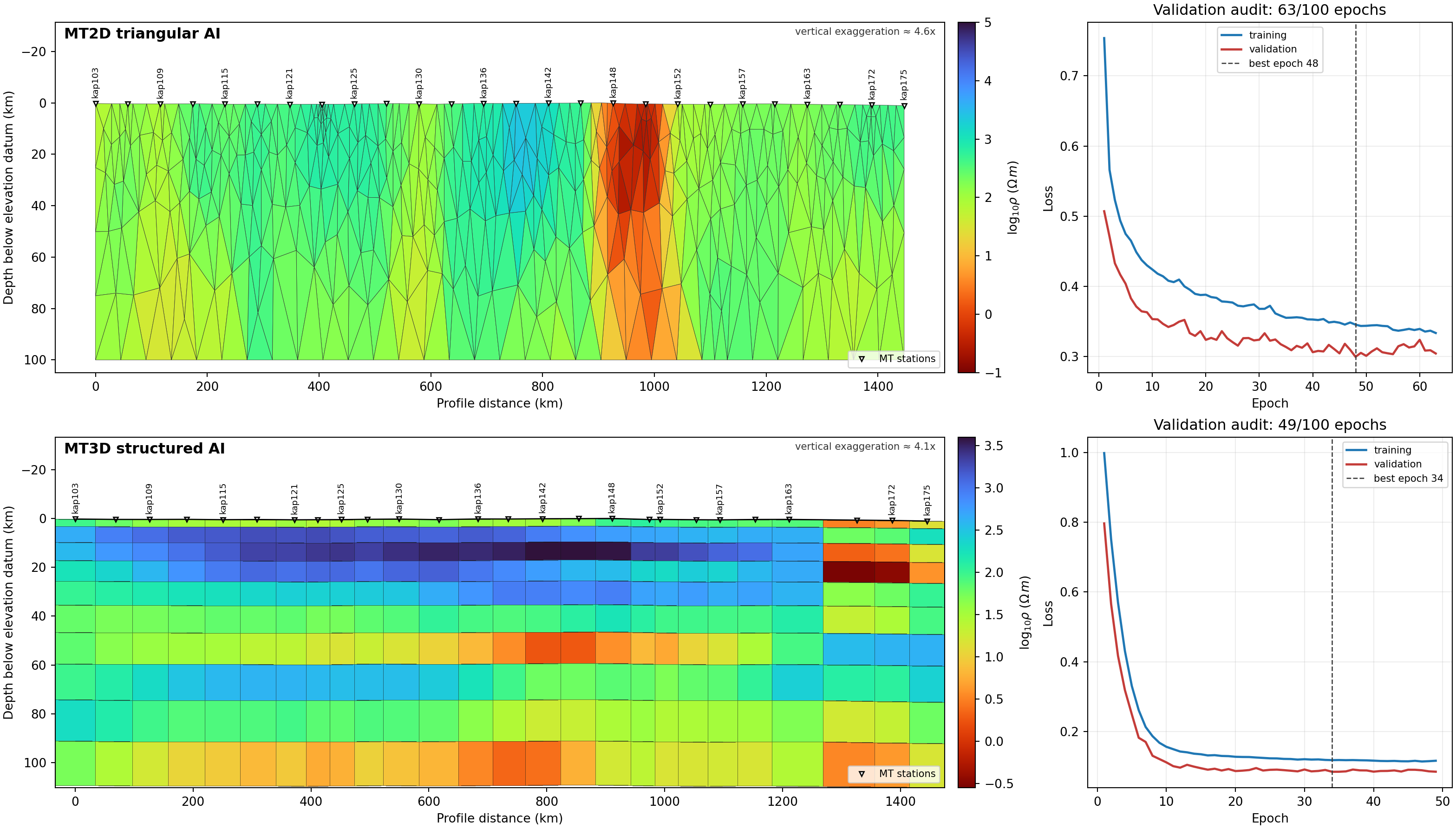
The first two columns of each row contain the inversion and the third contains
its actual epoch history. tripcolor preserves every MT2D triangle and its
edge, while pcolormesh exposes the station-by-depth cells of the MT3D
profile slice instead of smoothing them. The latter is a section through the
3-D prediction, not a claim that the full 3-D forward mesh is two-dimensional.
Both panels report their real, rendered vertical exaggeration in the top
corner (computed from the actual axes geometry at save time, not a fixed
assumption) – about 4.6x for MT2D and 4.1x for MT3D here. Compressing
100 km of depth and roughly 1,500 km of profile into a similarly
proportioned panel necessarily stretches every real feature vertically by
that factor; a companion small-scale MT2D triangular section from the
Process A TEMAVG Survey: TEM To Corrected EDI tutorial, plotted at its own natural ~1.7:1
aspect (600 m deep by 1,000 m wide) with no exaggeration to speak of,
confirms this same architecture produces smooth, laterally coherent
sections rather than “curtains” once the plot is not fighting a domain this
elongated – and, not incidentally, that example never hits the adjacency
bug described above either, because its 20 m mesh happens to sit
comfortably under Inv2DAgent’s 300 m default radius. Labelling the
exaggeration is the standard geological cross-section convention for
exactly this reason: it lets a reader separate real structure from a
plotting choice, rather than mistaking one for the other.
MT2D reaches its validation minimum at epoch 48 and stops after 15 further non-improving epochs, at epoch 63. MT3D reaches its minimum at epoch 34 and stops at epoch 49. Early stopping is active in both cases and restores the best checkpoint rather than retaining the final, more overfit weights.
The extrapolation failure that motivated the normalization fix was initially suspected to be mostly a real data-quality problem. Cross-checking which stations the extreme triangles clustered under, across three independent training runs before the normalization fix, found two stations – kap148 and kap169 – extreme in every run tested, which pointed at their real observed phase: kap148 spans -162.4° to +121.3° and kap169 spans -127.3° to +154.6°, both far outside the 0-90° range a minimum-phase impedance response should occupy (computed with pyCSAMT’s own convention, \(\rho_a=0.2f^{-1}|Z_{xy}|^2\), after catching and correcting a units error in an SI-based first attempt at this check). That diagnosis was not wrong exactly, but it was incomplete: it explained why those two stations’ already-unusual phase would be especially exposed by a normalization bug that gives every feature comparable weight regardless of scale, not that the anomaly required bad data to occur at all. Once normalization was fixed, the extreme-triangle count dropped from 143/660 to zero, including at kap148 and kap169. kap148 still stands out in the figure below – a real, localized low-resistivity feature reaching \(\log_{10}\rho \approx -0.6\) through much of the depth range beneath it – but that is now a physically plausible anomaly rather than a numerical blow-up, and it is consistent with kap148’s genuinely unusual phase rather than contradicting it. The other seed-dependent stations from the earlier cross-check (kap130, kap133, kap136, kap145, kap151, kap152, kap163, kap172) no longer show extreme triangles either.
The models are successful computational realizations, not yet defensible geological sections. Large adjacent resistivity contrasts and vertically coherent bands are more consistent with an underconstrained network and synthetic-to-field mismatch than with resolved lithosphere. The almost linear survey also supports only a narrow 3-D corridor, so off-profile structure is not resolved.
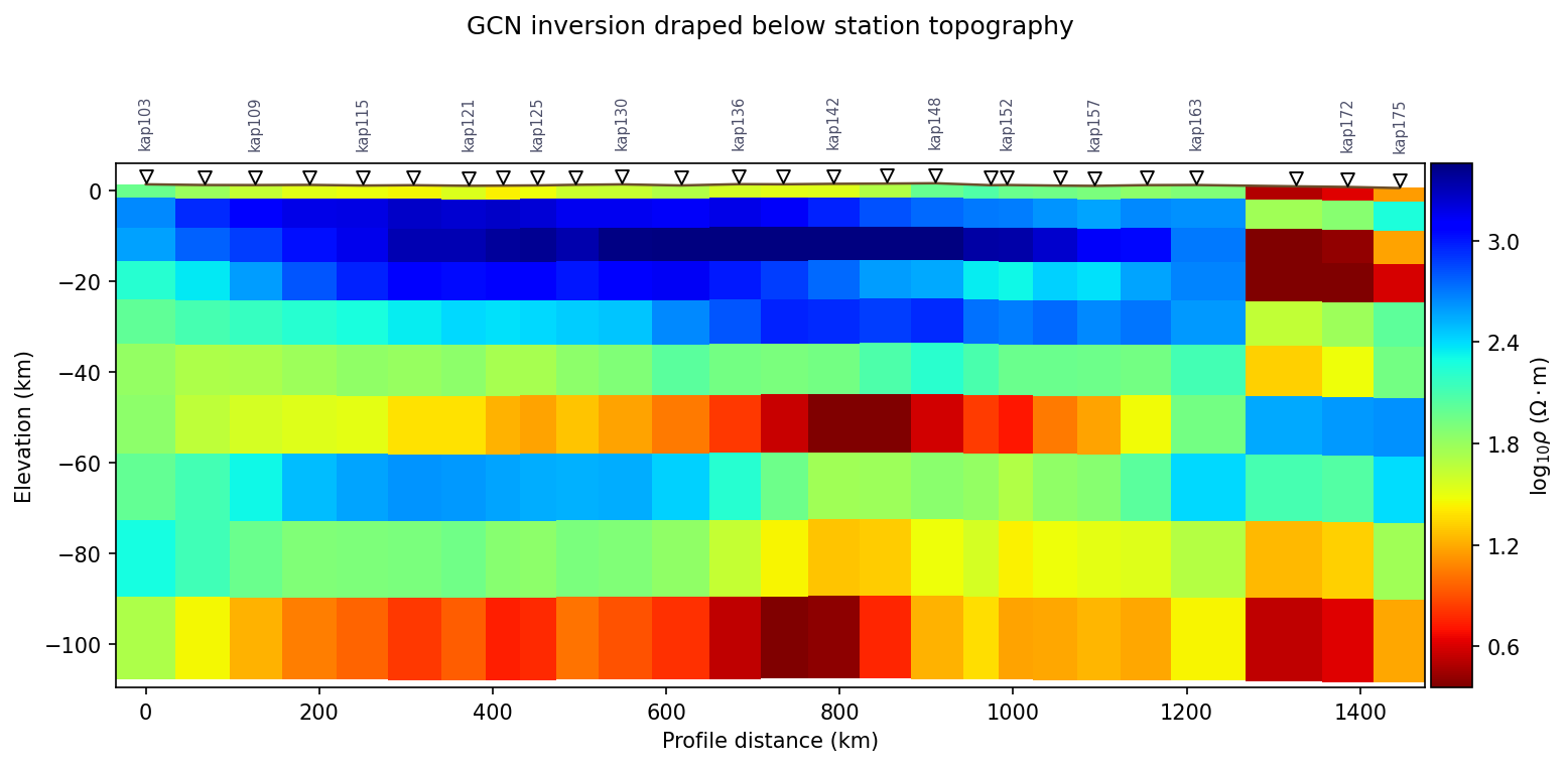
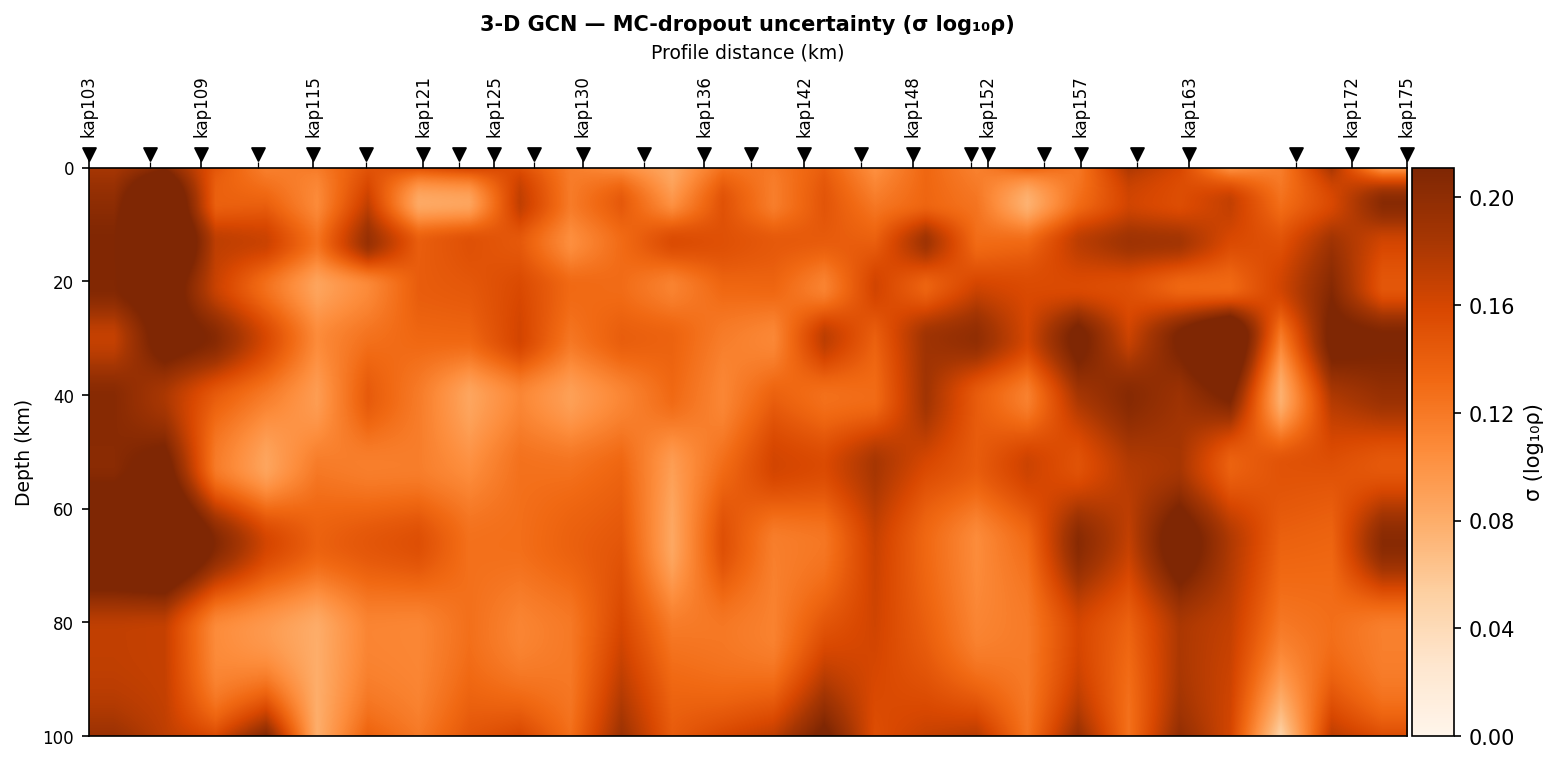
The topographic rendering places station markers at their EDI elevations, but the relief remains visually small compared with 100 km depth and still does not enter MT3D forward physics. MC-dropout uncertainty is typically 0.08-0.18 log-resistivity units across the section, reaching about 0.22 in the most uncertain patches (the shallow crust beneath KAP103, where the profile’s western end has fewer nearby stations to constrain it), so many apparent boundaries are not stable enough for geological picking.
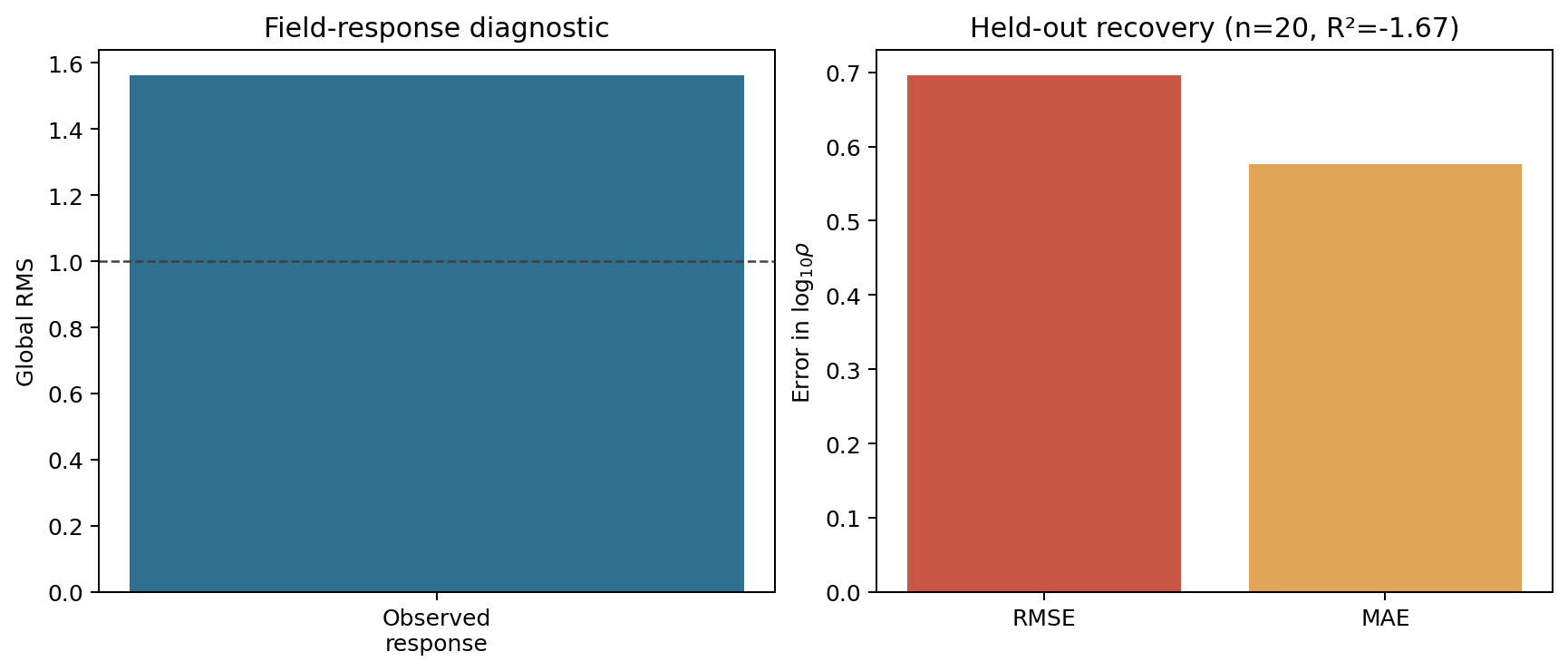
The MT3D observed-response RMS is 1.562, still above the unit-error target. Its held-out RMSE is 0.696 log units and \(R^2=-1.668\) over twenty held-out realizations – still meaning the predictor underperforms the held-out mean, unchanged from the earlier fine-mesh pass since this branch was not rerun here (the normalization bug affects it too – see above – but confirming the same fix helps MT3D’s own held-out recovery is future work, not something this pass measures). MT2D, with both fixes, now reaches RMSE 0.247 and \(R^2=0.726\) over the same twenty held-out realizations – clearly better than MT3D’s, and the best of every MT2D pass at this tutorial by a wide margin (0.337 at 100 realizations, 0.396 at 200 realizations with a coarse mesh, 0.349 at 200 realizations with a fine mesh but the depth-blind adjacency bug still present, 0.623 with the adjacency bug fixed but the normalization bug still present). That ordering is itself the useful result: mesh refinement alone made MT2D’s recovery worse (0.396 to 0.349), and it only improved once the two bugs present in every earlier number – neither of them something the mesh change introduced – were actually found and fixed. The lesson is not “finer mesh helps 2-D but not 3-D”; it is that MT2D’s real bottleneck was never mesh resolution, and no amount of mesh refinement was going to show it while the GCN could not use depth information at all, or while its own normalization was quietly discarding most of what it could use. More geological realizations, a larger validation/test allocation, bounded target resistivities, repeated seeds, and applying the same normalization fix’s benefit to MT3D are still required before either branch supports interpretation.
The runner stores its manifest under
results/kap03_mt_tutorial/inversion/ai_mt3d. Accept an AI result only when
the validation minimum precedes or coincides with the restored checkpoint,
held-out synthetic recovery is credible, observed-response RMS is reported,
and uncertainty does not dominate the interpreted target. A rising validation
curve followed by early stopping is expected evidence of overfitting control;
continuing to epoch 49 despite that rise would be the problematic behavior.
topography=True drapes the reported prediction and station markers over
the EDI elevations, but it does not change the present MT3D forward solve.
MT3DAdapter currently advertises supports_topography=False. The
triangular 2-D branch above is therefore the only mesh in this tutorial whose
forward-compatible surface actually follows elevation; claiming otherwise
would confuse visualization geometry with forward physics.
The triangular MT2D branch’s own configuration and execution code carries the adjacency-radius and mesh-size fix described above:
View the 100-epoch triangular MT2D execution codeClick to inspect and copy the complete code
 1def run_ai_mt2d_tri(sites, *, n_train_profiles: int = 20,
 2                    epochs: int = 50, patience: int = 8):
 3    """Run topography-following triangular MT2D training and field inference.
 4
 5    Shallower than the first pass at this tutorial (100 km instead of
 6    250 km -- KAP03's own frequency band, 5e-5 to 0.04 Hz, does not
 7    resolve structure anywhere near 250 km with useful confidence in the
 8    first place), but the surface/field cell sizes are now *finer* than
 9    both earlier passes: ``mesh_target_cell_m=15,000`` matches the
10    standalone display mesh built by :func:`build_profile_triangle_mesh`
11    rather than the coarser 45,000 m used previously, so the triangles
12    actually driving GCN training are no bigger than the ones already
13    shown as the "optional" mesh figure.
14
15    ``gcn_adjacency_radius_m`` is now set explicitly to 30,000 m (2x
16    ``mesh_target_cell_m``). It was never set in any earlier pass of
17    this tutorial, silently leaving ``Inv2DAgent``'s 300 m library
18    default in effect -- 15-40x smaller than the actual median distance
19    between neighbouring triangle centroids on this mesh (~10 km).
20    ``build_adjacency`` degrades to the identity matrix below that
21    distance, so the GCN never did any spatial message-passing in any
22    earlier run of this branch; every triangle nearest a given station
23    predicted the same value regardless of its own depth, which is what
24    produced the flat vertical "curtain" per station visible in the
25    comparison figure before this fix.
26    """
27    from pycsamt.agents import Inv2DAgent
28    from pycsamt.forward.maxwell.tri_fem2d import TriFEM2DAdapter
29
30    chain, surface_depth = profile_geometry()
31    n_sites = len(list(sites))
32    spacing = float(chain[-1] / max(n_sites - 1, 1))
33    np.random.seed(23)
34    try:
35        import torch
36
37        torch.manual_seed(23)
38    except ImportError:
39        pass
40    agent = Inv2DAgent(
41        physics="mt2d_tri",
42        epochs=epochs,
43        patience=patience,
44        n_freqs=8,
45        depth_max=100_000.0,
46        n_train_profiles=n_train_profiles,
47        n_stations_per_profile=n_sites,
48        station_spacing_m=spacing,
49        mesh_target_cell_m=15_000.0,
50        field_grid_cell_m=7_500.0,
51        gcn_adjacency_radius_m=30_000.0,
52        correlation_length_x_m=(40_000.0, 180_000.0),
53        correlation_length_z_m=(5_000.0, 25_000.0),
54        gcn_hidden=(128, 64, 32),
55        topo_x_m=chain,
56        topo_z_m=surface_depth,
57        mare2dem_adapter=TriFEM2DAdapter(),
58    )
59    AI2D_DIR.mkdir(parents=True, exist_ok=True)
60    result = agent.execute({
61        "sites": sites,
62        "freqs": np.geomspace(5.0e-5, 0.04, 8),
63        "output_dir": str(AI2D_DIR),
64    })
65    if result.status != "success":
66        raise RuntimeError(result.summary)
67    recovery = result.data.get("mt2d_tri_recovery") or {}
68    history = result.data.get("training_history") or {}
69    pred = result.data["pred_triangles"]
70    station_x = np.arange(n_sites, dtype=float) * spacing
71    station_names = np.array([s.station for s in sites])
72    np.savez_compressed(
73        AI2D_DIR / "mesh_prediction.npz",
74        nodes_m=np.asarray(pred["mesh"].nodes_m),
75        triangles=np.asarray(pred["mesh"].triangles),
76        log10_resistivity=np.asarray(pred["log10_resistivity"]),
77        station_x_m=station_x,
78        station_z_m=np.interp(station_x, chain, surface_depth),
79        station_names=station_names,
80    )
81    manifest = {
82        "status": result.status,
83        "epochs_requested": epochs,
84        "early_stopping_patience": patience,
85        "training_realizations": n_train_profiles,
86        "epochs_completed": int(result.data.get("epochs_completed", 0)),
87        "best_validation_loss": float(result.data.get("best_validation_loss", np.nan)),
88        "held_out_recovery": recovery,
89        "training_history": history,
90    }
91    (AI2D_DIR / "run_manifest.json").write_text(
92        json.dumps(manifest, indent=2, default=float), encoding="utf-8"
93    )
94    print(json.dumps(manifest, indent=2, default=float))
95    return result
The structured-mesh MT3D branch is set up the same way, on its own mesh and station adjacency:
View the 100-epoch MT3D AI configuration and execution codeClick to inspect and copy the complete code
 1def run_ai_mt3d(sites, *, n_train_profiles: int = 20, epochs: int = 50, patience: int = 8):
 2    """Run the structured-mesh MT3D training branch on request.
 3
 4    Shallower than the first pass, for the same reason as
 5    :func:`run_ai_mt2d_tri`: 100 km depth instead of 250 km. The lever
 6    that actually thins the *plotted* MT3D section is ``n_layers`` (10
 7    depth rows instead of 6; the 26 station columns are already the
 8    real station count and cannot be finer) -- ``geology_grid_nx_ny``,
 9    ``geology_grid_nz``, and ``max_mesh_cells`` instead control the
10    realism/cost of the *training-data* forward solves and were left
11    close to their original values on purpose. Two smoke tests found a
12    real 3-D Maxwell solve's cost on this solver scales far worse than
13    linearly with cell count: quadrupling ``max_mesh_cells`` to 20,000
14    multiplied per-realization time by ~17x (not 4x), and even a modest
15    5,000-to-8,000 bump (with ``geology_grid_nx_ny=4``,
16    ``geology_grid_nz=5``) multiplied it by ~5.8x -- a 200-realization
17    run at that setting would take about 5.4 hours, not the ~2-2.5
18    hours a naive N^2 estimate suggested. ``max_mesh_cells=6,000``
19    (a 20% bump) with the original ``geology_grid_nx_ny=3``,
20    ``geology_grid_nz=4`` keeps training-data cost close to the
21    original run's while still giving every realization a slightly
22    finer solver core.
23    """
24    from pycsamt.agents import Inv3DAgent
25
26    np.random.seed(17)
27    try:
28        import torch
29
30        torch.manual_seed(17)
31    except ImportError:
32        pass
33    agent = Inv3DAgent(
34        physics="mt3d",
35        n_layers=10,
36        freqs=np.geomspace(5.0e-5, 0.04, 8),
37        depth_max=100_000.0,
38        n_train_profiles=n_train_profiles,
39        epochs=epochs,
40        patience=patience,
41        radius=120_000.0,
42        hidden=(128, 64, 32),
43        dropout=0.1,
44        n_mc=20,
45        correlation_length_x_m=(40_000.0, 180_000.0),
46        correlation_length_y_m=(40_000.0, 150_000.0),
47        correlation_length_z_m=(5_000.0, 25_000.0),
48        geology_grid_nx_ny=3,
49        geology_grid_nz=4,
50        mesh_safety_factor=8.0,
51        max_mesh_cells=6_000,
52    )
53    result = agent.execute({
54        "sites": sites,
55        "topography": True,
56        "output_dir": str(AI_DIR),
57    })
58    if result.status != "success":
59        raise RuntimeError(result.summary)
60    recovery = result.data.get("mt3d_recovery") or {}
61    station_names = np.array([s.station for s in sites])
62    manifest = {
63        "status": result.status,
64        "epochs_requested": epochs,
65        "early_stopping_patience": patience,
66        "training_realizations": n_train_profiles,
67        "rms_global": float(result.data["rms_global"]),
68        "held_out_recovery": recovery,
69        "epochs_completed": int(result.data.get("epochs_completed", 0)),
70        "best_validation_loss": float(result.data.get("best_validation_loss", np.nan)),
71        "training_history": result.data.get("training_history") or {},
72    }
73    AI_DIR.mkdir(parents=True, exist_ok=True)
74    (AI_DIR / "run_manifest.json").write_text(json.dumps(manifest, indent=2, default=float), encoding="utf-8")
75    np.savez_compressed(
76        AI_DIR / "mesh_prediction.npz",
77        log10_resistivity=np.asarray(result.data["pred_rho"]),
78        depths_km=np.asarray(result.data["depths_km"]),
79        chainage_km=np.asarray(result.data.get("station_chainage_km")),
80        elevation_m=np.asarray(result.data.get("station_elevation_m")),
81        station_names=station_names,
82    )
83    print(json.dumps(manifest, indent=2, default=float))
84    return result
Both results feed the same two-row comparison-and-validation figure shown above:
View the two-row inversion and validation-grid codeClick to inspect and copy the complete code
  1def plot_ai_comparison(mt2d_result=None, mt3d_result=None):
  2    """Make the requested 2 x 3 inversion/validation comparison."""
  3    rows = [
  4        ("MT2D triangular AI", AI2D_DIR / "mesh_prediction.npz",
  5         AI2D_DIR / "run_manifest.json", mt2d_result),
  6        ("MT3D structured AI", AI_DIR / "mesh_prediction.npz",
  7         AI_DIR / "run_manifest.json", mt3d_result),
  8    ]
  9    if not all(mesh_path.exists() and manifest_path.exists()
 10               for _, mesh_path, manifest_path, _ in rows):
 11        return
 12    fig = plt.figure(figsize=(16.5, 9.4), constrained_layout=True)
 13    gs = fig.add_gridspec(2, 3, width_ratios=(1.0, 1.0, 0.82))
 14    model_axes = []
 15    for row, (title, mesh_path, manifest_path, result) in enumerate(rows):
 16        ax_model = fig.add_subplot(gs[row, :2])
 17        model_axes.append(ax_model)
 18        mesh_data = np.load(mesh_path)
 19        if row == 0:
 20            import matplotlib.tri as mtri
 21
 22            nodes = mesh_data["nodes_m"] / 1000.0
 23            triangulation = mtri.Triangulation(
 24                nodes[:, 0], nodes[:, 1], mesh_data["triangles"]
 25            )
 26            # Clip the *display* range only -- a handful of triangles
 27            # nearest a few far-profile stations (real, uncorrected field
 28            # apparent resistivity/phase well outside anything the
 29            # synthetic training distribution ever produced) extrapolate
 30            # to physically nonsensical log10(rho) values in the tens; a
 31            # few such outliers would otherwise wash out the legitimate
 32            # depth-varying structure across the rest of the section.
 33            # ``log10_resistivity`` in the saved .npz is untouched.
 34            clip_lo, clip_hi = -1.0, 5.0
 35            log_rho = mesh_data["log10_resistivity"]
 36            n_clipped = int(np.sum((log_rho < clip_lo) | (log_rho > clip_hi)))
 37            artist = ax_model.tripcolor(
 38                triangulation, facecolors=log_rho,
 39                cmap="turbo_r", shading="flat", edgecolors="0.18",
 40                linewidth=0.28, vmin=clip_lo, vmax=clip_hi,
 41            )
 42            ax_model.plot(mesh_data["station_x_m"] / 1000.0,
 43                          mesh_data["station_z_m"] / 1000.0,
 44                          "kv", ms=4, mfc="white", label="MT stations")
 45            ax_model.set(xlabel="Profile distance (km)",
 46                         ylabel="Depth below elevation datum (km)")
 47            ax_model.invert_yaxis()
 48            ax_model.legend(loc="lower right", fontsize=8)
 49            if n_clipped:
 50                ax_model.text(
 51                    0.99, 0.02,
 52                    f"{n_clipped}/{log_rho.size} triangles off-scale"
 53                    f" (clipped to [{clip_lo:g}, {clip_hi:g}])",
 54                    transform=ax_model.transAxes, ha="right", va="bottom",
 55                    fontsize=7.5, color="0.25",
 56                    bbox={"facecolor": "white", "edgecolor": "none",
 57                          "alpha": 0.75, "pad": 1.5},
 58                )
 59            if "station_names" in mesh_data:
 60                _add_station_labels(
 61                    ax_model,
 62                    mesh_data["station_x_m"] / 1000.0,
 63                    mesh_data["station_z_m"] / 1000.0,
 64                    mesh_data["station_names"],
 65                )
 66        else:
 67            values = mesh_data["log10_resistivity"].T
 68            x = mesh_data["chainage_km"]
 69            z = mesh_data["depths_km"]
 70            x_edges = _centres_to_edges(x)
 71            z_edges = _centres_to_edges(z, lower_bound=0.0)
 72            elevation = mesh_data["elevation_m"]
 73            surface_depth = (np.nanmax(elevation) - elevation) / 1000.0
 74            surface_edges = _centres_to_edges(surface_depth)
 75            x_grid = np.broadcast_to(x_edges[None, :],
 76                                     (z_edges.size, x_edges.size))
 77            z_grid = z_edges[:, None] + surface_edges[None, :]
 78            artist = ax_model.pcolormesh(
 79                x_grid, z_grid, values, cmap="turbo_r", shading="flat",
 80                edgecolors=(0.08, 0.08, 0.08, 0.55), linewidth=0.32,
 81            )
 82            ax_model.plot(x, surface_depth, "k-", lw=1.0, zorder=4)
 83            ax_model.plot(x, surface_depth, "kv", ms=4, mfc="white",
 84                          label="MT stations")
 85            ax_model.set(xlabel="Profile distance (km)",
 86                         ylabel="Depth below elevation datum (km)")
 87            ax_model.invert_yaxis()
 88            ax_model.legend(loc="lower right", fontsize=8)
 89            if "station_names" in mesh_data:
 90                _add_station_labels(ax_model, x, surface_depth, mesh_data["station_names"])
 91        fig.colorbar(
 92            artist, ax=ax_model, pad=0.015,
 93            extend="both" if (row == 0 and n_clipped) else "neither",
 94            label=r"$\log_{10}\rho$ ($\Omega\,m$)",
 95        )
 96        ax_model.text(
 97            0.01, 0.985, title, transform=ax_model.transAxes,
 98            ha="left", va="top", fontsize=12, fontweight="bold",
 99            bbox={"facecolor": "white", "edgecolor": "none", "alpha": 0.78,
100                  "pad": 2.0}, zorder=8,
101        )
102        audit = json.loads(manifest_path.read_text(encoding="utf-8"))
103        history = ((result.data.get("training_history") or {}) if result
104                   else (audit.get("training_history") or {}))
105        ax_loss = fig.add_subplot(gs[row, 2])
106        train = np.asarray(history.get("train_loss", []), dtype=float)
107        valid = np.asarray(history.get("val_loss", []), dtype=float)
108        if train.size:
109            ax_loss.plot(np.arange(1, train.size + 1), train, color="#1f77b4",
110                         lw=1.8, label="training")
111        if valid.size:
112            ax_loss.plot(np.arange(1, valid.size + 1), valid, color="#c43c39",
113                         lw=1.8, label="validation")
114            best = int(np.nanargmin(valid)) + 1
115            ax_loss.axvline(best, color="0.25", ls="--", lw=1.0,
116                            label=f"best epoch {best}")
117        completed = int(audit.get("epochs_completed", max(train.size, valid.size)))
118        requested = int(audit.get("epochs_requested", 50))
119        ax_loss.set(xlabel="Epoch", ylabel="Loss",
120                    title=f"Validation audit: {completed}/{requested} epochs")
121        ax_loss.grid(alpha=0.22)
122        if train.size or valid.size:
123            ax_loss.legend(fontsize=8)
124
125    # Both model panels compress ~100 km of depth into roughly the same
126    # on-screen width as ~1,500 km of profile -- real, close-to-isotropic
127    # triangles (independently verified: median width/height ratio 0.99 on
128    # the MT2D mesh) therefore render visibly "tall." Rather than let that
129    # read as a mesh defect, compute the actual exaggeration from the
130    # rendered axes geometry (not an assumed constant) and label it
131    # explicitly, the same disclosure convention geological cross-sections
132    # use for any vertically exaggerated section.
133    fig.canvas.draw()
134    for ax_model in model_axes:
135        bbox_in = ax_model.get_window_extent().transformed(
136            fig.dpi_scale_trans.inverted()
137        )
138        xlim = ax_model.get_xlim()
139        ylim = ax_model.get_ylim()
140        data_w = abs(xlim[1] - xlim[0])
141        data_h = abs(ylim[1] - ylim[0])
142        km_per_in_x = data_w / bbox_in.width
143        km_per_in_y = data_h / bbox_in.height
144        vert_exag = km_per_in_x / km_per_in_y
145        ax_model.text(
146            0.99, 0.985, f"vertical exaggeration ≈ {vert_exag:.1f}x",
147            transform=ax_model.transAxes, ha="right", va="top", fontsize=8,
148            color="0.2",
149            bbox={"facecolor": "white", "edgecolor": "none", "alpha": 0.78,
150                  "pad": 1.8}, zorder=8,
151        )
152    fig.savefig(IMAGE_DIR / "kp_ai_mt2d_mt3d_comparison.png", dpi=190)
153    plt.close(fig)
18.6.17. Processing Decision Table#
Summarise the choices before writing processed EDIs:
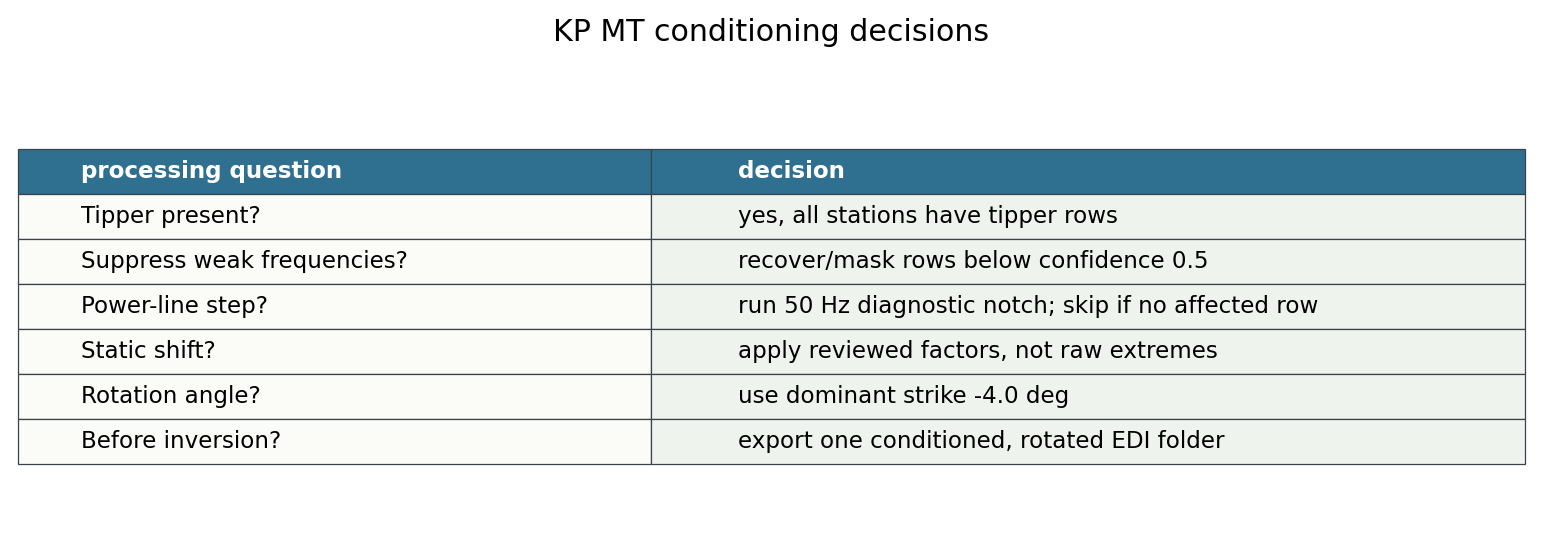
For a production run, save:
the raw QC tables;
the weak-frequency table;
the rejected static-shift trial and its rationale;
the strike estimate and rotation angle;
the processed EDI folder;
a short note explaining any rejected stations or frequency bands.
18.6.18. Adapting This Tutorial#
For your own MT data, change only the input folder and representative station names first:
>>> edi_dir = Path("path/to/your/mt_edis")
>>> stations_to_plot = ["S001", "S010", "S020", "S030"]
Then rerun the same sequence. If the survey lacks tipper, skip the tipper plots but keep the tensor, QC, static-shift, phase-tensor, and rotation steps. If the strike rose is broad or multimodal, do not force a single rotation angle; split the line into domains or keep the original coordinate frame.
18.6.19. See Also#
- Inspect and QC a Survey
One-line QC tables and confidence diagnostics.
- Correct Static Shift
Conservative static-shift correction workflow.
- Prepare an Occam2D Inversion
Prepare inversion files after the line has been conditioned.
- Prepare A ModEM Inversion
Detailed ModEM file, mesh, covariance, execution, and result checks.
- AI Inversion From Corrected EDIs
Expanded AI geology, training, validation, uncertainty, and plotting guide.
- Run a Pipeline From Config
Move stable processing decisions into a reusable config file.