18.14. AI Inversion From Corrected EDIs

This tutorial starts where the processing tutorials end: you already have a folder of corrected EDI files and you want to use AI inversion instead of, or alongside, a classical Occam2D, ModEM, or MARE2DEM run. It runs the complete, real pipeline end to end on one survey — loading, auditing, a geological prior, a 2-D Maxwell training mesh, a 2-D AI inversion, a 3-D AI inversion, real station topography, and an out-of-distribution check — and reports what actually came out, including the parts that did not work well.

The survey is K2: Line 2 of a real Chinese CSAMT exploration line (station prefix Z2HX), 86 corrected EDI files, a magnetotelluric acquisition with a cross-sounding array at 20 m station spacing per its own field log, 29 frequencies per station spanning 15.8 Hz–10 kHz, and real station coordinates and elevation:

k2_corrected/

Static shift, near-field, and coordinate corrections of the kind EM Tools Guide’s diagnostics pages cover are assumed already applied. K2 is intentionally not bundled with pyCSAMT — replace the path with your own exported corrected EDI folder, for example results/L18PLT_first_qc/processed, to repeat every step here on your own survey.

18.14.1. What You Will Learn

After this tutorial you should be able to:

• audit a corrected survey’s dimensionality, geoelectric strike consistency, frequency-grid, and station-coordinate quality before choosing an inversion path, not after;

• ground a geological prior’s resistivity range in the survey’s own apparent resistivity instead of guessing one;

• build a real 2-D Maxwell training mesh and dataset sized to the survey’s actual station spacing and extent;

• run Inv2DAgent’s physics="mt2d" 2-D AI inversion and read its automatic held-out recovery check;

• run Inv3DAgent’s graph-convolutional 3-D AI inversion from real station coordinates, with Monte Carlo dropout uncertainty;

• drape a prediction below real station topography, and know that this is a display correction, not new forward physics;

• catch a confidently wrong prediction with an out-of-distribution screen before a plausible-looking figure is mistaken for a validated one.

18.14.2. Reproducibility before the private case study

K2 is not distributed with pyCSAMT, so the figure generator separates portable and survey-specific work. Geological composition, mesh construction, the Maxwell training pair, and the following learning audit run without K2. The audit uses eight stations from bundled data/AMT/WILLY_data/L18PLT and the same Inv2DAgent API. It is deliberately small—24 profiles and eight epochs—so it verifies installation and exposes the result contract; it is not a scientifically accepted inversion.

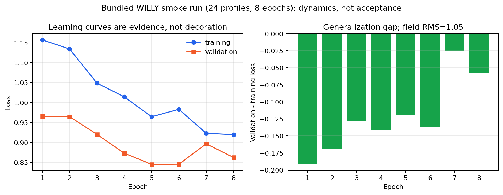
Executed, portable learning audit on bundled corrected EDIs.

Validation loss below training loss in this short run is possible because the training objective sees augmentation and mini-batch variability while a tiny validation split can be easier by chance. It is not evidence that the model generalizes unusually well. The important observations are that both curves are retained, neither has stabilized convincingly in eight epochs, and the field RMS is reported independently. A production decision requires repeated seeds and held-out recovery, not a preferred curve shape from one smoke run.

</>View and copy the bundled smoke-run codeClick to inspect and copy the complete code

def make_training_convergence_smoke() -> None:
    """Run a small bundled-data fit so tutorial readers can audit learning dynamics."""
    from pycsamt.agents import Inv2DAgent
    from pycsamt.emtools._core import ensure_sites

    sites = ensure_sites(ROOT / "data" / "AMT" / "WILLY_data" / "L18PLT",
                         recursive=True, verbose=0).ordered()
    names = [site.name for site in sites][:8]
    subset = sites.select(names=names).ordered()
    frequencies = np.logspace(0, 3, 10)
    result = Inv2DAgent(
        physics="mt1d", n_depth=12, n_stations_per_profile=8,
        n_train_profiles=24, epochs=8, depth_max=1200,
        api_key=None,
    ).execute({"sites": subset, "freqs": frequencies})
    if result.status != "success":
        raise RuntimeError(result.error)
    history = result.data["inverter"]._history
    train = np.asarray(history["train_loss"])
    valid = np.asarray(history["val_loss"])
    epochs = np.arange(1, len(train) + 1)
    fig, axes = plt.subplots(1, 2, figsize=(10.8, 4.2))
    axes[0].plot(epochs, train, "o-", label="training", color="#2563eb")
    axes[0].plot(epochs, valid, "s-", label="validation", color="#f15a29")
    axes[0].set(xlabel="Epoch", ylabel="Loss", title="Learning curves are evidence, not decoration")
    axes[0].grid(alpha=0.25)
    axes[0].legend(frameon=False)
    gap = valid - train
    axes[1].bar(epochs, gap, color=np.where(gap > 0, "#dc2626", "#16a34a"))
    axes[1].axhline(0, color="#111827", lw=1)
    axes[1].set(xlabel="Epoch", ylabel="Validation - training loss",
                title=f"Generalization gap; field RMS={result.data['rms_global']:.2f}")
    axes[1].grid(alpha=0.25, axis="y")
    fig.suptitle("Bundled WILLY smoke run (24 profiles, 8 epochs): dynamics, not acceptance", fontsize=12)
    fig.tight_layout()
    _save(fig, "training_convergence_smoke.png")

Run the complete generator with

python docs/scripts/generate_tutorial_ai_inversion.py

When k2_corrected is absent, it writes the portable figures and explicitly skips only the K2 audit and inversion figures. Replace K2_DIR with your corrected EDI directory to execute the survey-specific path.

18.14.3. Load and Audit the Survey

Loading a corrected EDI folder is one call:

>>> from pycsamt.emtools._core import ensure_sites
>>> sites = ensure_sites(
...     "k2_corrected", recursive=False, verbose=0
... ).ordered()
>>> print("stations:", len(sites))
stations: 86
>>> print("ordering applied:", sites.ordering["applied"])
ordering applied: chainage
>>> print("profile linearity:", round(sites.ordering["linearity"], 5))
profile linearity: 0.99998
>>> print("profile span (m):", round(sites.ordering["span_m"], 1))
profile span (m): 1635.7

ordered() confirms K2 is a clean, nearly perfectly linear 1636 m profile before anything else runs — but a linear profile is not the same as a survey ready for a fixed-axis 2-D or per-station AI inversion. audit_survey() checks that directly:

>>> from pycsamt.ai.domain_gap import audit_survey
>>> report = audit_survey(sites, verbose=0)
>>> print("frequency grid matched:", report.frequency_grid.matched)
frequency grid matched: False
>>> print(
...     "stations with a different grid:",
...     len(report.frequency_grid.mismatched_stations),
... )
stations with a different grid: 53
>>> print(
...     "station spacing (m):",
...     {k: round(v, 2) for k, v in report.station_spacing_m.items()},
... )
station spacing (m): {'min': 0.0, 'median': 19.94, 'max': 41.32}
>>> dim = report.dimensionality
>>> print("dimensionality samples:", dim.n_samples)
dimensionality samples: 2208
>>> print(
...     "fraction 1-D / 2-D / 3-D:",
...     round(dim.frac_1d, 4), round(dim.frac_2d, 4), round(dim.frac_3d, 4),
... )
fraction 1-D / 2-D / 3-D: 0.0082 0.0942 0.8976
>>> print(
...     "strike consensus / IQR (deg):",
...     round(dim.strike_consensus_deg, 2),
...     round(dim.strike_consensus_iqr_deg, 2),
... )
strike consensus / IQR (deg): -9.36 84.39
>>> print(
...     "stations recommending 3-D review:",
...     len(dim.stations_recommending_3d_review),
... )
stations recommending 3-D review: 86
>>> print("static shift log10 sigma:", round(report.static_shift_log10_sigma, 4))
static shift log10 sigma: 0.3943
>>> print(
...     "distortion twist sigma (deg):",
...     round(report.distortion_twist_deg_sigma, 2),
... )
distortion twist sigma (deg): 35.03

Four real findings come out of this before a single inversion has run:

• The median 19.94 m station spacing matches the field log’s declared 20 m point spacing almost exactly — a genuine, independent confirmation that the corrected coordinates are trustworthy.

• The minimum spacing of 0.0 m is not trustworthy: at least one pair of stations shares an identical coordinate. K2 turns out to have four — Z2HX042/Z2HX043, Z2HX068/Z2HX069, Z2HX074/Z2HX075, and Z2HX086/Z2HX087 — most likely a repeat occupation recorded under two station names.

• 53 of 86 stations do not share the reference station’s exact frequency set; FrequencyGridReport’s per-station counts range from 8 to 29 across the line, so a workflow that assumes one common frequency axis (as the sections below do) is already resampling, not just reading, most of this survey.

• Nearly 90% of K2’s station-period samples classify as dimensionality 3-D, barely 1% as 1-D, and every one of the 86 stations is flagged for a 3-D review by pre2d_inversion_assessment(). The geoelectric strike estimate is not a clean, sharp azimuth either: a median of -9.36° sounds precise until its 84° interquartile spread shows individual stations disagreeing with each other almost as much as they possibly could.

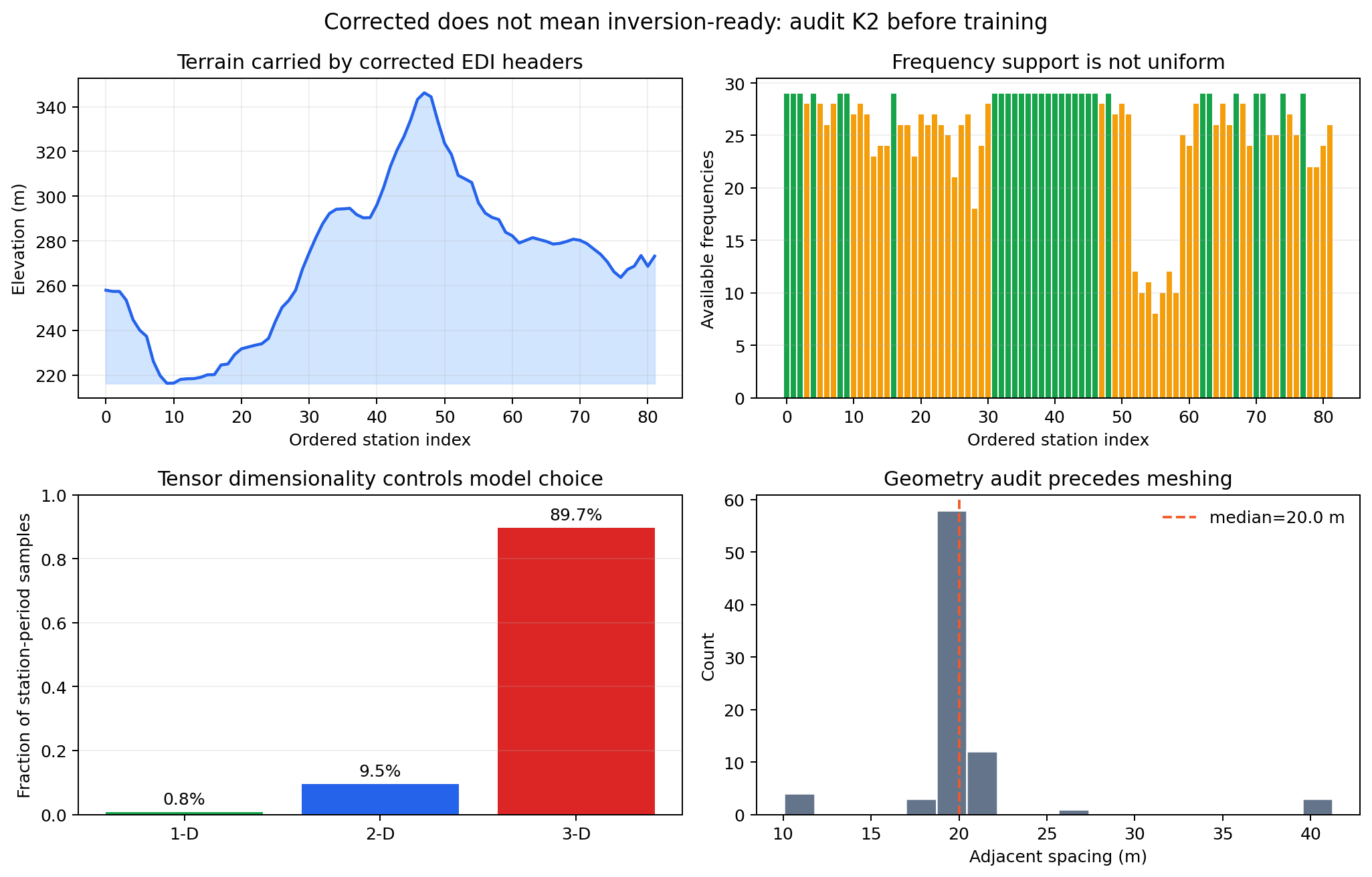
Four pre-inversion checks computed from the corrected EDI collection.

The panels make the decision problem visible. Elevation is smooth enough to define a credible terrain profile, whereas frequency support changes sharply near stations 50–60 and must be resampled with masks retained. The dominant 3-D classification is not a small minority of suspect periods; it controls the dimensionality decision. Finally, the tight spacing peak verifies the nominal acquisition interval after duplicate coordinates have been removed. No model architecture can repair these issues after training: they determine the data contract and admissible physics before training begins.

</>View and copy the survey-audit figure codeClick to inspect and copy the complete code

def make_survey_audit() -> None:
    """Visualize the K2 geometry, frequency coverage, and dimensionality gate."""
    from pycsamt.ai.domain_gap import audit_survey

    sites = _k2_clean_sites()
    report = audit_survey(sites, verbose=0)
    names = [site.name for site in sites]
    elevations = np.array([site.coords[2] for site in sites], dtype=float)
    counts = np.array([len(site.freq) for site in sites], dtype=int)
    dim = report.dimensionality
    fractions = np.array([dim.frac_1d, dim.frac_2d, dim.frac_3d])
    lat = np.array([site.coords[0] for site in sites], dtype=float)
    lon = np.array([site.coords[1] for site in sites], dtype=float)
    lat0 = np.radians(np.nanmean(lat))
    dx = np.diff(lon) * 111_320.0 * np.cos(lat0)
    dy = np.diff(lat) * 110_574.0
    spacing = np.sqrt(dx**2 + dy**2)

    fig, axes = plt.subplots(2, 2, figsize=(11.5, 7.4))
    index = np.arange(len(sites))
    axes[0, 0].plot(index, elevations, color="#2563eb", lw=1.8)
    axes[0, 0].fill_between(index, elevations.min(), elevations,
                            color="#bfdbfe", alpha=0.7)
    axes[0, 0].set(xlabel="Ordered station index", ylabel="Elevation (m)",
                   title="Terrain carried by corrected EDI headers")
    axes[0, 0].grid(alpha=0.2)
    axes[0, 1].bar(index, counts, color=np.where(counts == counts.max(), "#16a34a", "#f59e0b"))
    axes[0, 1].set(xlabel="Ordered station index", ylabel="Available frequencies",
                   title="Frequency support is not uniform")
    axes[0, 1].grid(alpha=0.2, axis="y")
    axes[1, 0].bar(["1-D", "2-D", "3-D"], fractions,
                   color=["#16a34a", "#2563eb", "#dc2626"])
    axes[1, 0].set(ylim=(0, 1), ylabel="Fraction of station-period samples",
                   title="Tensor dimensionality controls model choice")
    for i, value in enumerate(fractions):
        axes[1, 0].text(i, value + 0.025, f"{value:.1%}", ha="center")
    axes[1, 0].grid(alpha=0.2, axis="y")
    axes[1, 1].hist(spacing[np.isfinite(spacing)], bins=18, color="#64748b",
                    edgecolor="white")
    axes[1, 1].axvline(report.station_spacing_m["median"], color="#f15a29",
                       ls="--", label=f"median={report.station_spacing_m['median']:.1f} m")
    axes[1, 1].set(xlabel="Adjacent spacing (m)", ylabel="Count",
                   title="Geometry audit precedes meshing")
    axes[1, 1].legend(frameon=False)
    fig.suptitle("Corrected does not mean inversion-ready: audit K2 before training", fontsize=13)
    fig.tight_layout()
    _save(fig, "survey_audit.png")

None of the sections below rotate the tensor into that (barely consistent) strike frame — zxy and zyx are used exactly as the EDI files store them, which is also what Inv2DAgent and Inv3DAgent do internally. Strike rotation is what would normally separate a clean TE response from a clean TM response at a station whose local strike differs from the survey’s nominal direction; skip it, and a component literally named zxy is under no obligation to behave like the “TE-like” curve either agent’s training data was built to expect. That single sentence is the mechanical explanation for most of what the rest of this tutorial finds. The duplicate stations are dropped before anything downstream needs a strictly increasing chainage:

>>> lat = [s.coords[0] for s in sites]
>>> lon = [s.coords[1] for s in sites]
>>> names = [s.name for s in sites]
>>> keep = [names[0]]
>>> last = (lat[0], lon[0])
>>> for i in range(1, len(names)):
...     if (lat[i], lon[i]) == last:
...         continue
...     keep.append(names[i])
...     last = (lat[i], lon[i])
...
>>> clean = sites.select(names=keep).ordered()
>>> print("clean stations:", len(clean))
clean stations: 82

18.14.4. Ground a Geological Prior in the Survey

Correlated geological priors and 2-D Maxwell training-data generation need a log_resistivity_mean/log_resistivity_std pair for the synthetic training realizations. Guessing one is not necessary when the survey itself already reports an apparent resistivity:

>>> import numpy as np
>>> rho_xy = np.concatenate([s.rho[:, 0, 1] for s in sites])
>>> rho_yx = np.concatenate([s.rho[:, 1, 0] for s in sites])
>>> rho_all = np.concatenate([rho_xy, rho_yx])
>>> rho_all = rho_all[np.isfinite(rho_all) & (rho_all > 0)]
>>> print(
...     "median apparent resistivity (ohm.m):",
...     round(float(np.median(rho_all)), 1),
... )
median apparent resistivity (ohm.m): 117.3
>>> print(
...     "log10 mean / std:",
...     round(float(np.log10(rho_all).mean()), 4),
...     round(float(np.log10(rho_all).std()), 4),
... )
log10 mean / std: 1.9456 1.2342

The survey’s own median apparent resistivity of 117 Ω·m puts log_resistivity_mean=2.0 (100 Ω·m) within a few percent of the data, rather than an arbitrary round number. Its raw log-spread of 1.23 decades is not copied directly into log_resistivity_std, though: apparent resistivity smears every depth and every local distortion into one frequency-indexed curve, so its spread always overstates the true resistivity variability a geological prior should target. log_resistivity_std=0.5 — roughly half the raw spread — is the conservative choice used for both inversions below.

That statistical range still does not define geology. A robust prior must state which units occupy which depths, how interfaces vary laterally, and how terrain divides air from earth. The complete figure code below constructs three electrical units, correlated interface relief, an interpolated TopographicSurface, and a padded solver mesh.

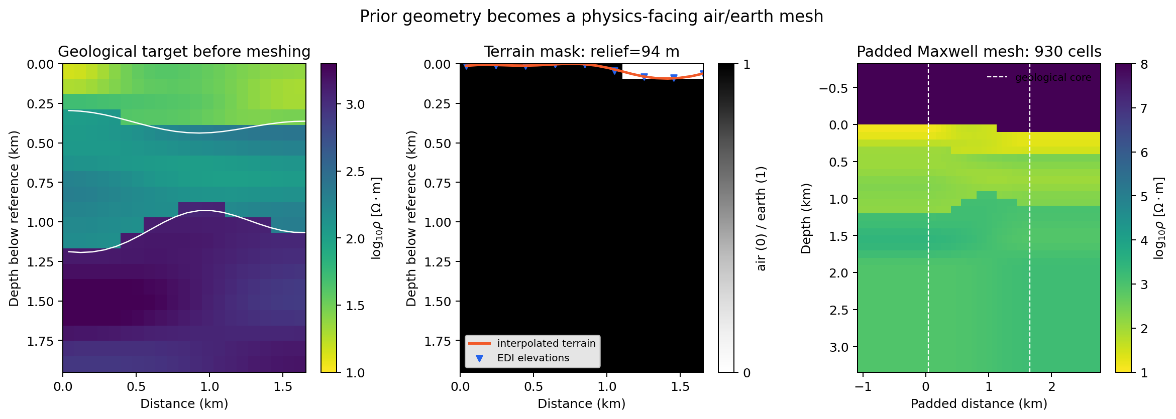
The same model at three successive contracts: geological target, terrain mask, and physics-facing padded mesh.

The left panel is the supervised target, not a prediction: its white curves are stochastic interfaces and its within-unit variation follows declared correlation lengths. In the middle panel, station elevations become a continuous surface and a Boolean air/earth mask; interpolation is therefore a modelling choice with provenance, not merely a plotting option. The right panel adds five air, five bottom-padding, and five padding cells on each side. The dark air is assigned a small numerical conductivity rather than rock resistivity.

The mesh is intentionally diagnostic. Its 930 cells resolve the smallest skin depth with only 0.298 core cells, while MeshDesign requests four. Therefore solver.quality.acceptable is false and its warning must not be ignored. The dataset builder used for the figure below refines this geometry to 39,776 cells; the separately seeded sample in the executable block reaches 58,052. The padded count can change with the realization’s resistivity extrema because they change the skin-depth requirement. This is why geological-grid resolution and Maxwell-solver resolution are related but not interchangeable.

</>View and copy the geology, topography, and mesh codeClick to inspect and copy the complete code

def make_geology_topography_mesh() -> None:
    """Build the tutorial prior, terrain surface, and padded solver mesh."""
    from pycsamt.ai.geology import (
        ElectricalLayer,
        GaussianCorrelation,
        GeologyGrid,
        generate_layered_geology,
        interpolate_topography,
    )
    from pycsamt.forward.maxwell.mesh import MeshDesign, build_solver_mesh

    grid = GeologyGrid.regular_2d(nx=21, nz=20, dx_m=80.8, dz_m=100.0)
    layers = (
        ElectricalLayer("conductive cover", 35.0, log10_std=0.12,
                        heterogeneity=GaussianCorrelation(350, 100)),
        ElectricalLayer("weathered host", 140.0, log10_std=0.16,
                        heterogeneity=GaussianCorrelation(500, 160)),
        ElectricalLayer("resistive basement", 1200.0, log10_std=0.10,
                        heterogeneity=GaussianCorrelation(700, 220)),
    )
    geology = generate_layered_geology(
        grid, layers, [380.0, 1050.0], seed=17,
        interface_relief_std_m=[45.0, 90.0],
        interface_correlation=GaussianCorrelation(550, 150),
        minimum_thickness_m=120.0,
    )
    control_x = np.linspace(grid.x_m[0], grid.x_m[-1], 9)
    elevation = 285 + 42 * np.sin(control_x / 310) + 18 * np.cos(control_x / 145)
    topography = interpolate_topography(
        grid, control_x, elevation, source="corrected EDI elevations",
        interpolation_method="cubic",
    )
    solver = build_solver_mesh(
        grid, resistivity_ohm_m=geology.resistivity_ohm_m,
        frequencies_hz=[15.8, 10_000.0], topography=topography,
        design=MeshDesign(horizontal_padding_cells=5, bottom_padding_cells=5,
                          air_layers=5),
    )

    fig, axes = plt.subplots(1, 3, figsize=(13.2, 4.7))
    extent = (0, grid.x_m[-1] / 1000, grid.z_m[-1] / 1000, 0)
    image = axes[0].imshow(np.log10(geology.resistivity_ohm_m), extent=extent,
                           aspect="auto", cmap="viridis_r", vmin=1, vmax=3.3)
    for interface in geology.interface_depth_m:
        axes[0].plot(grid.x_m / 1000, interface / 1000, "w-", lw=1)
    axes[0].set(title="Geological target before meshing", xlabel="Distance (km)",
                ylabel="Depth below reference (km)")
    fig.colorbar(image, ax=axes[0], label=r"$\log_{10}\rho$ [$\Omega\cdot$m]")

    topo_image = axes[1].imshow(topography.earth_mask(), extent=extent,
                                aspect="auto", cmap="Greys", vmin=0, vmax=1)
    axes[1].plot(grid.x_m / 1000, topography.surface_depth_m / 1000,
                 color="#f15a29", lw=2, label="interpolated terrain")
    axes[1].scatter(control_x / 1000,
                    topography.surface_depth_m[np.searchsorted(grid.x_m, control_x)] / 1000,
                    marker="v", color="#2563eb", s=24, label="EDI elevations")
    axes[1].set(title=f"Terrain mask: relief={topography.relief_m:.0f} m",
                xlabel="Distance (km)", ylabel="Depth below reference (km)")
    axes[1].legend(facecolor="white", framealpha=0.9, fontsize=8,
                   loc="lower left")
    fig.colorbar(topo_image, ax=axes[1], ticks=[0, 1], label="air (0) / earth (1)")

    x_edges = solver.mesh.x_edges_m / 1000
    z_edges = solver.mesh.z_edges_m / 1000
    mesh_values = np.log10(1.0 / solver.conductivity_s_m)
    mesh_image = axes[2].pcolormesh(x_edges, z_edges, mesh_values,
                                    shading="flat", cmap="viridis_r", vmin=1, vmax=8)
    axes[2].set(title=f"Padded Maxwell mesh: {solver.quality.cell_count:,} cells",
                xlabel="Padded distance (km)", ylabel="Depth (km)")
    axes[2].invert_yaxis()
    axes[2].axvline(grid.x_m[0] / 1000, color="white", ls="--", lw=0.9)
    axes[2].axvline(grid.x_m[-1] / 1000, color="white", ls="--", lw=0.9,
                    label="geological core")
    axes[2].legend(frameon=False, fontsize=8)
    fig.colorbar(mesh_image, ax=axes[2], label=r"$\log_{10}\rho$ [$\Omega\cdot$m]")
    fig.suptitle("Prior geometry becomes a physics-facing air/earth mesh", fontsize=13)
    fig.tight_layout()
    _save(fig, "geology_topography_mesh.png")

18.14.5. Build the Training Mesh and 2-D Maxwell Dataset

Maxwell2DDatasetConfig turns a GeologyGrid sized to the real profile — 82 clean stations span 1616 m, a 2 km depth target is more than generous for a 15.8 Hz–10 kHz CSAMT band — into a mesh and a batch of solved realizations, exactly as 2-D Maxwell training-data generation describes:

>>> from pycsamt.ai.geology import GeologyGrid
>>> from pycsamt.ai.training.dataset2d import (
...     Maxwell2DDatasetConfig,
...     generate_2d_maxwell_dataset,
... )
>>> grid = GeologyGrid.regular_2d(
...     nx=21, nz=20, dx_m=1616.36 / 20, dz_m=2000.0 / 20
... )
>>> config = Maxwell2DDatasetConfig(
...     dataset_id="k2-tutorial",
...     grid=grid,
...     correlation_length_x_m=(200.0, 600.0),
...     correlation_length_z_m=(50.0, 200.0),
...     frequencies_hz=[
...         15.8, 31.6, 63.1, 126.0, 251.0,
...         501.0, 1000.0, 2000.0, 3980.0, 7940.0,
...     ],
...     station_x_m=grid.x_m,
...     n_realizations=1,
...     seed=0,
...     log_resistivity_mean=2.0,
...     log_resistivity_std=0.5,
...     components=("zxy",),
...     validation_fraction=0.0,
...     test_fraction=0.0,
... )
>>> dataset = generate_2d_maxwell_dataset(config)
>>> sample = dataset.samples[0]
>>> print("mesh cells:", sample.mesh_cells)
mesh cells: 58052
>>> print("relative residual:", round(sample.relative_residual, 12))
relative residual: 0.0
>>> print(
...     "resistivity range (ohm.m):",
...     round(float(sample.resistivity_ohm_m.min()), 1),
...     round(float(sample.resistivity_ohm_m.max()), 1),
... )
resistivity range (ohm.m): 4.6 2534.0

The single training-pair diagnostic above uses ten frequencies and a 21-station geometry so its mesh can be inspected quickly. The inversion below keeps the same ten-frequency teaching band but regenerates the Maxwell dataset for all 82 unique-coordinate stations. These remain Solver-neutral Maxwell contracts and 2-D Maxwell training-data generation demonstration settings, not a claim that ten frequencies or 24 realizations are sufficient for production. The single realization above already exercises the real pipeline: 58,052 mesh cells, a relative residual essentially at floating-point zero, and a resistivity range that comfortably contains the survey’s own 117 Ω·m median.

Before generating hundreds of realizations, inspect one complete supervised pair. The target is the earth model on the left; apparent resistivity and phase on the right are derived from the solved complex impedance and become the network input. They are not alternative images of the target: Maxwell physics smooths and mixes subsurface structure in a frequency-dependent way.

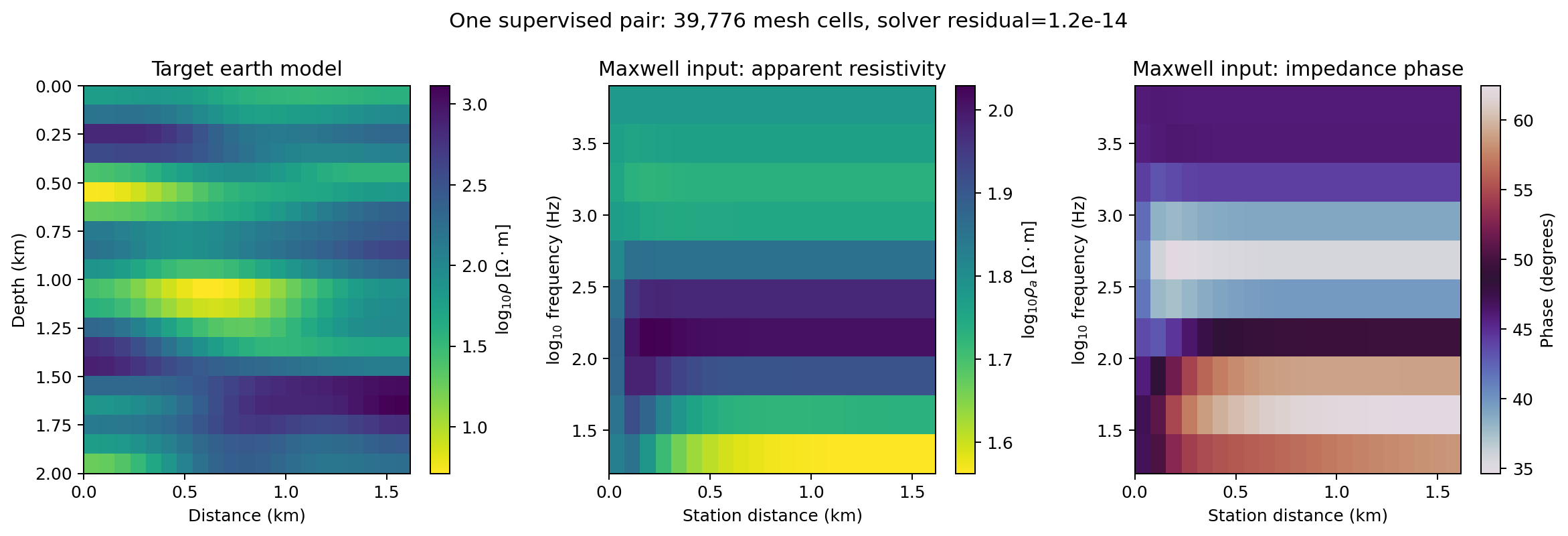
One deterministic 2-D Maxwell training pair using the tutorial geometry and frequency band.

The conductive body near 1.1 km depth produces a broad response rather than a cell-for-cell copy, while high frequencies are dominated by shallower structure. Phase contributes information that apparent resistivity alone does not preserve. The reported residual of approximately \(1.2\times10^{-14}\) is the linear-solver residual; it demonstrates that the discrete system converged, not that the mesh is free from discretization or boundary error. Those require the independent benchmarks described in Solver-neutral Maxwell contracts.

</>View and copy the solved training-pair codeClick to inspect and copy the complete code

def make_maxwell_training_pair() -> None:
    """Generate one solved 2-D training pair and expose model/response structure."""
    from pycsamt.ai.geology import GeologyGrid
    from pycsamt.ai.training.dataset2d import Maxwell2DDatasetConfig, generate_2d_maxwell_dataset

    grid = GeologyGrid.regular_2d(nx=21, nz=20, dx_m=80.8, dz_m=100.0)
    frequencies = np.array([15.8, 31.6, 63.1, 126, 251, 501, 1000, 2000, 3980, 7940])
    config = Maxwell2DDatasetConfig(
        dataset_id="corrected-edi-tutorial-figure", grid=grid,
        correlation_length_x_m=(200.0, 600.0),
        correlation_length_z_m=(50.0, 200.0), frequencies_hz=frequencies,
        station_x_m=grid.x_m, n_realizations=1, seed=23,
        log_resistivity_mean=2.0, log_resistivity_std=0.5,
        components=("zxy",), validation_fraction=0, test_fraction=0,
    )
    sample = generate_2d_maxwell_dataset(config).samples[0]
    impedance = sample.survey.impedance[:, :, 0]
    mu0 = 4e-7 * np.pi
    apparent = np.abs(impedance) ** 2 / (2 * np.pi * frequencies[None, :] * mu0)
    phase = np.angle(impedance, deg=True)

    fig, axes = plt.subplots(1, 3, figsize=(13.2, 4.5))
    image = axes[0].imshow(np.log10(sample.resistivity_ohm_m), aspect="auto",
                           extent=(0, 1.616, 2.0, 0), cmap="viridis_r")
    axes[0].set(title="Target earth model", xlabel="Distance (km)", ylabel="Depth (km)")
    fig.colorbar(image, ax=axes[0], label=r"$\log_{10}\rho$ [$\Omega\cdot$m]")
    for ax, values, title, label, cmap in (
        (axes[1], np.log10(apparent).T, "Maxwell input: apparent resistivity",
         r"$\log_{10}\rho_a$ [$\Omega\cdot$m]", "viridis_r"),
        (axes[2], phase.T, "Maxwell input: impedance phase", "Phase (degrees)", "twilight"),
    ):
        response_image = ax.imshow(values, origin="lower", aspect="auto",
                                   extent=(0, 1.616, np.log10(frequencies[0]),
                                           np.log10(frequencies[-1])), cmap=cmap)
        ax.set(xlabel="Station distance (km)", ylabel=r"$\log_{10}$ frequency (Hz)",
               title=title)
        fig.colorbar(response_image, ax=ax, label=label)
    fig.suptitle(f"One supervised pair: {sample.mesh_cells:,} mesh cells, "
                 f"solver residual={sample.relative_residual:.1e}", fontsize=12.5)
    fig.tight_layout()
    _save(fig, "maxwell_training_pair.png")

18.14.6. Run 2-D AI Inversion

Inv2DAgent wraps exactly the steps above — build the mesh, generate realizations, train, predict on the real pseudosection — behind the physics="mt2d" execution contract introduced in Architecture roadmap:

>>> import numpy as np
>>> from pycsamt.agents import Inv2DAgent
>>> print("raw EDI sites / unique-coordinate sites:", len(sites), len(clean))
raw EDI sites / unique-coordinate sites: 86 82
>>> freqs = np.array([
...     15.8, 31.6, 63.1, 126.0, 251.0,
...     501.0, 1000.0, 2000.0, 3980.0, 7940.0,
... ])
>>> agent = Inv2DAgent(
...     physics="mt2d",
...     n_depth=20,
...     n_stations_per_profile=len(clean),
...     n_train_profiles=24,
...     epochs=30,
...     depth_max=2000.0,
...     station_spacing_m=20.2,
...     correlation_length_x_m=(200.0, 600.0),
...     correlation_length_z_m=(50.0, 200.0),
...     log_resistivity_mean=2.0,
...     log_resistivity_std=0.5,
...     lambda_x=0.01,
...     lambda_z=0.005,
...     lambda_tv=0.002,
...     mesh_safety_factor=4.0,
... )
>>> result = agent.execute({
...     "sites": clean,
...     "freqs": freqs,
...     "topography": True,
... })
>>> print("status:", result.status)
status: success
>>> print("global RMS:", round(result.data["rms_global"], 3))
global RMS: 2.106
>>> recovery = {
...     key: round(value, 3) if isinstance(value, float) else value
...     for key, value in result.data["mt2d_recovery"].items()
... }
>>> print("held-out recovery:", recovery)
held-out recovery: {'rmse': 0.518, 'mae': 0.418, 'r2': -0.075, 'n_samples': 2}

station_spacing_m=20.2 is the median spacing of the 82 distinct station coordinates. The directory currently contains 86 EDI files, but four pairs occupy identical coordinates; retaining both members of a pair would create zero-length cells and duplicate observations at one abscissa. The earlier demonstration selected every fourth clean station and therefore showed only 21 markers. That decimation has been removed from the primary result. mesh_safety_factor=4 keeps this executed tutorial near a three-minute runtime; it reduces the lateral domain margin from the package default of eight and is not a production choice until the mesh-sensitivity benchmark passes for the survey band. For a full run, generate and cache the larger Maxwell dataset offline with the default safety factor, then train repeatedly without resolving every realization.

Training loss must be inspected before the predicted section. The fitted inverter remains available in the result, so the numerical history is not hidden inside the agent:

>>> history = result.data["inverter"]._history
>>> sorted(history)
['train_loss', 'val_loss']
>>> len(history["train_loss"]), len(history["val_loss"])
(13, 13)

Early stopping ended this captured run after thirteen of the requested thirty epochs. Requesting thirty epochs is an upper bound, not evidence that thirty updates were useful. The exact curves change because the agent does not yet expose a training seed; the executed figure and held-out verdict must be archived together for each run.

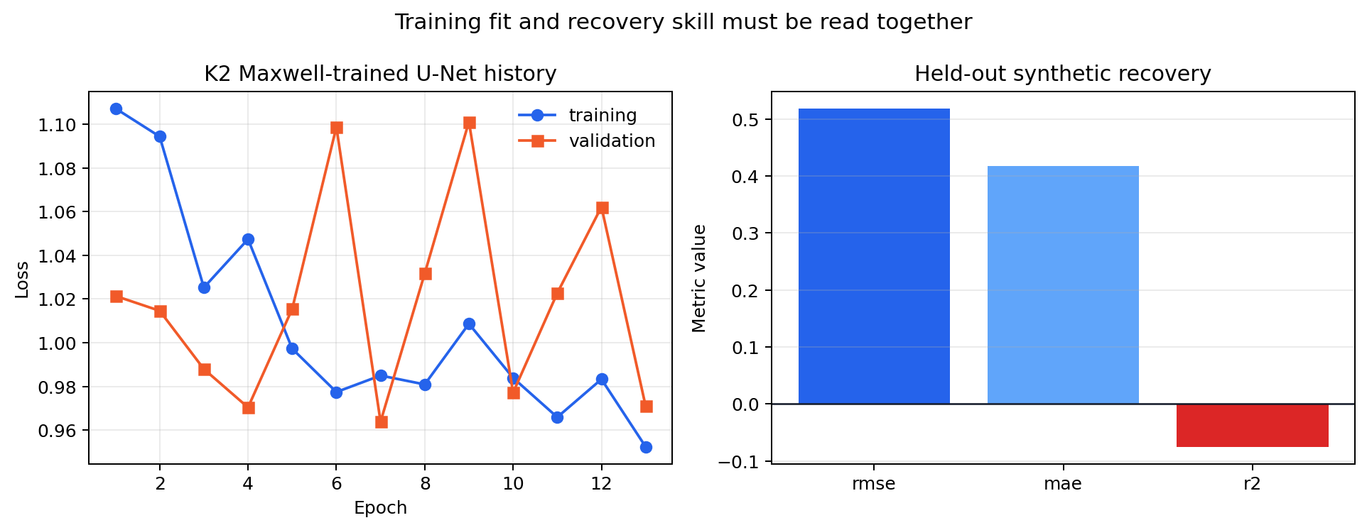
Executed K2 learning curves and held-out synthetic recovery from the same physics="mt2d" run.

Training loss trends downward while validation loss oscillates strongly after the fourth epoch. That gap is the onset of memorizing a tiny 24-realization training set. The right panel reaches the more important conclusion: on all 82 unique-coordinate stations, field RMS rises to 2.106 and the prediction extends from -2.47 to 5.25 in log-resistivity. Held-out \(R^2=-0.075\) is worse than predicting the target mean. The full-line result is therefore a transparent demonstration-scale failure, not an accepted interpretation. Increasing epochs alone would deepen the gap. Cache a larger set of independent Maxwell realizations, repeat seeds, and re-evaluate an untouched test partition.

</>View the complete 2-D run and diagnostic-figure codeClick to inspect and copy the complete code

def make_inv2d_topography() -> None:
    """Real physics="mt2d" Inv2DAgent run on all 82 unique K2 stations."""
    from pycsamt.agents import Inv2DAgent

    clean = _k2_clean_sites()
    freqs = _K2_FULL_FREQS_HZ[::3]
    agent = Inv2DAgent(
        physics="mt2d",
        n_depth=20,
        n_stations_per_profile=len(clean),
        n_train_profiles=24,
        epochs=30,
        depth_max=2000.0,
        station_spacing_m=20.2,
        correlation_length_x_m=(200.0, 600.0),
        correlation_length_z_m=(50.0, 200.0),
        log_resistivity_mean=2.0,
        log_resistivity_std=0.5,
        lambda_x=0.01,
        lambda_z=0.005,
        lambda_tv=0.002,
        mesh_safety_factor=4.0,
    )
    result = agent.execute({"sites": clean, "freqs": freqs, "topography": True})
    if result.status == "failed":
        raise RuntimeError(result.error)
    fig = result["figures"]["topography_section"]
    _save(fig, "inv2d_topography_section.png")
    print(
        "K2 2-D:",
        {"rms_global": result.data["rms_global"],
         "recovery": result.data.get("mt2d_recovery"),
         "log10_rho_range": (
             float(np.nanmin(result.data["pred_section"])),
             float(np.nanmax(result.data["pred_section"])),
         )},
    )
    history = result.data["inverter"]._history
    train = np.asarray(history["train_loss"])
    valid = np.asarray(history["val_loss"])
    epoch = np.arange(1, len(train) + 1)
    fig, axes = plt.subplots(1, 2, figsize=(10.8, 4.2))
    axes[0].plot(epoch, train, "o-", color="#2563eb", label="training")
    axes[0].plot(epoch, valid, "s-", color="#f15a29", label="validation")
    axes[0].set(xlabel="Epoch", ylabel="Loss", title="K2 Maxwell-trained U-Net history")
    axes[0].grid(alpha=0.25)
    axes[0].legend(frameon=False)
    recovery = result.data.get("mt2d_recovery") or {}
    metric_names = ["rmse", "mae", "r2"]
    metric_values = [float(recovery.get(name, np.nan)) for name in metric_names]
    axes[1].bar(metric_names, metric_values,
                color=["#2563eb", "#60a5fa", "#dc2626"])
    axes[1].axhline(0, color="#111827", lw=1)
    axes[1].set(ylabel="Metric value", title="Held-out synthetic recovery")
    axes[1].grid(alpha=0.25, axis="y")
    fig.suptitle("Training fit and recovery skill must be read together", fontsize=12.5)
    fig.tight_layout()
    _save(fig, "inv2d_training_and_recovery.png")

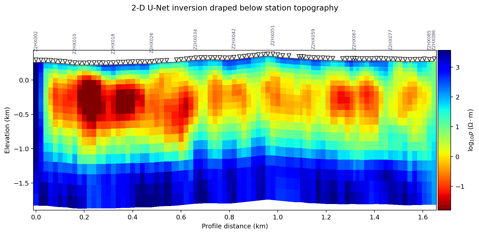
physics="mt2d" U-Net section for all 82 unique-coordinate K2 stations, draped below the line’s own elevation.

Every inverted station is represented by a downward triangle. Only a readable subset of station names is printed by the shared station-rendering preset; those labels are ticks for orientation, not the list of stations used by the inversion. Thus 82 markers and model columns are present even though only about a dozen names are visible.

The section visibly follows the real terrain — the drape comes from topography=True resolving each station’s own elevation and chainage, exactly as resolve_agent_topography() documents. What the numbers say is more sobering than the figure alone. mt2d_recovery is recovery_report() run on a held-out synthetic realization with known truth — see Recovery, residual, and OOD diagnostics for what this check computes and why Inv2DAgent already calls it automatically whenever physics="mt2d" has a held-out split to check against — and at only 24 training realizations its \(R^2\) is negative: worse than predicting the mean, on a sample of two held-out realizations too small to be conclusive on its own but entirely consistent with training on two dozen realizations rather than the “hundreds to thousands… a training dataset needs” that Architecture roadmap states plainly is the realistic scale for a genuine Maxwell-solved training set. This is exactly the number recovery_report() exists to surface before a fast section is mistaken for a validated one. Re-running this exact block will not reproduce these digits bit for bit — neither agent pins a training seed. The corrected full-line geometry exposes rather than repairs the weak recovery: negative \(R^2\), an RMS above two log decades, and extreme resistivities are rejection evidence. This section is a diagnostic candidate, not a released earth model.

18.14.7. Run 3-D AI Inversion

Inv3DAgent takes a structurally different path: rather than a genuinely 2-D Maxwell solve, it tiles independent 1-D forward models across every station and lets a graph convolutional network share information between neighbours within a configurable radius, as AI inversion agents describes. It reads real per-station coordinates from the EDI headers directly, so the full 82-station clean line can be used at once:

>>> import numpy as np
>>> from pycsamt.agents import Inv3DAgent
>>> lat = np.array([s.coords[0] for s in clean])
>>> lon = np.array([s.coords[1] for s in clean])
>>> elevation_m = np.array([s.coords[2] for s in clean])
>>> lat0 = np.radians(lat[0])
>>> x_m = (lon - lon[0]) * 111_320.0 * np.cos(lat0)
>>> y_m = (lat - lat[0]) * 110_574.0
>>> seg_m = np.sqrt(np.diff(x_m) ** 2 + np.diff(y_m) ** 2)
>>> chainage_km = np.concatenate([[0.0], np.cumsum(seg_m)]) / 1000.0
>>> freqs_full = np.array([
...     15.8, 20.0, 25.1, 31.6, 39.8, 50.1, 63.1, 79.4, 100.0,
...     126.0, 158.0, 200.0, 251.0, 316.0, 398.0, 501.0, 631.0,
...     794.0, 1000.0, 1260.0, 1580.0, 2000.0, 2510.0, 3160.0,
...     3980.0, 5010.0, 6310.0, 7940.0, 10000.0,
... ])
>>> agent3d = Inv3DAgent(
...     n_layers=6,
...     epochs=30,
...     n_train_profiles=150,
...     n_mc=20,
...     radius=300.0,
...     depth_max=2000.0,
... )
>>> result3d = agent3d.execute({
...     "sites": clean,
...     "freqs": freqs_full,
...     "topography": {
...         "elevation_m": elevation_m,
...         "chainage_km": chainage_km,
...     },
... })
>>> off_diag = (result3d.data["adjacency"] > 0).sum(axis=1) - 1
>>> print("status:", result3d.status)
status: success
>>> print(
...     "mean / min / max neighbours:",
...     round(float(off_diag.mean()), 2),
...     int(off_diag.min()),
...     int(off_diag.max()),
... )
mean / min / max neighbours: 20.24 11 24
>>> print("global RMS:", round(result3d.data["rms_global"], 3))
global RMS: 8.02

freqs_full is all 29 real K2 frequencies here — the tiled 1-D solves an Inv3DAgent run needs are far cheaper per realization than a 2-D Maxwell mesh, so the full band is affordable. elevation_m and chainage_km are supplied explicitly (computed from clean’s own ordered coordinates) rather than left to the default sites-derived extraction, because that extraction requires a strictly increasing chainage and would otherwise refuse to render on the same duplicate-coordinate stations already dropped above. A radius of 300 m against a ~20 m median spacing connects each station to roughly twenty neighbours on either side — dense enough for the GCN to average across real local noise, not so dense that the graph collapses to one node.

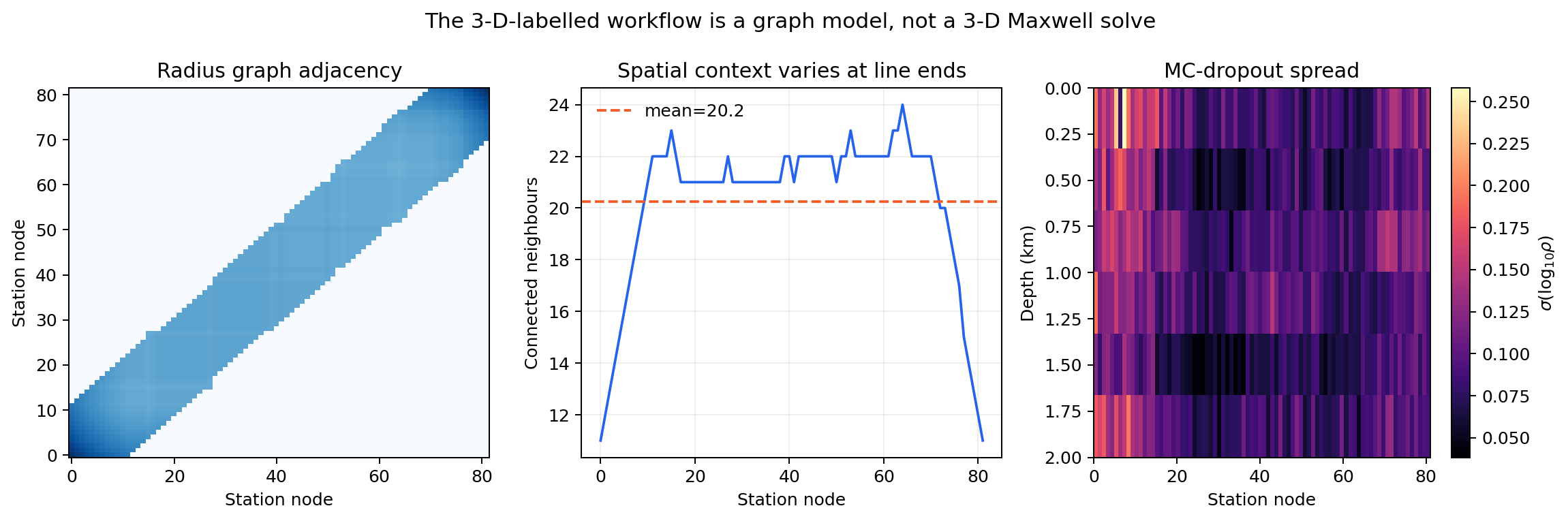
Internal spatial graph and predictive spread from the executed Inv3DAgent run.

The banded adjacency matrix confirms that information travels along nearby stations, while end stations have fewer neighbours and therefore a different context from central nodes. The uncertainty panel is smooth and small, but it is conditional on this graph model and its tiled 1-D training physics. It does not turn the workflow into a 3-D Maxwell inversion. Calling this output “3-D” describes the spatial graph and output organization; the forward model remains the limitation stated in Architecture roadmap.

</>View the complete graph and uncertainty diagnostic codeClick to inspect and copy the complete code

def make_inv3d_graph_diagnostic() -> None:
    """Real Inv3DAgent (GCN) run on the full 82-station clean K2 line."""
    from pycsamt.agents import Inv3DAgent

    clean = _k2_clean_sites()
    lat = np.array([s.coords[0] for s in clean])
    lon = np.array([s.coords[1] for s in clean])
    elev = np.array([s.coords[2] for s in clean])
    lat0 = np.radians(lat[0])
    x_m = (lon - lon[0]) * 111_320.0 * np.cos(lat0)
    y_m = (lat - lat[0]) * 110_574.0
    chain_km = np.concatenate(
        [[0.0], np.cumsum(np.sqrt(np.diff(x_m) ** 2 + np.diff(y_m) ** 2))]
    ) / 1000.0
    agent = Inv3DAgent(
        n_layers=6, epochs=30, n_train_profiles=150, n_mc=20,
        radius=300.0, depth_max=2000.0,
    )
    result = agent.execute({
        "sites": clean,
        "freqs": _K2_FULL_FREQS_HZ,
        "topography": {"elevation_m": elev, "chainage_km": chain_km},
    })
    if result.status == "failed":
        raise RuntimeError(result.error)
    raw_log_rho = np.asarray(result.data["pred_rho"])
    physical = np.isfinite(raw_log_rho) & (raw_log_rho >= 0.0) & (raw_log_rho <= 5.0)
    bounded_log_rho = np.where(physical, raw_log_rho, np.nan)
    from pycsamt.topo import plot_topo_section

    rejected_model = {
        "pred_rho": bounded_log_rho,
        "depths_km": result.data["depths_km"],
        "station_names": result.data["station_names"],
        "rms_global": result.data["rms_global"],
    }
    ax = plot_topo_section(
        rejected_model,
        elevation=elev,
        chainage=chain_km,
        station_names=result.data["station_names"],
        station_x=chain_km,
        topo_source="array",
        model_unit="km",
        depth_max=2.0,
        title="Rejected GCN candidate: only physically bounded cells are shown",
    )
    ax.text(
        0.5, 0.96,
        f"REJECTED — {100 * (1 - physical.mean()):.1f}% of cells outside "
        r"$1$–$10^5\ \Omega\,\mathrm{m}$ display bounds",
        transform=ax.transAxes, ha="center", va="top", color="white",
        fontsize=10, fontweight="bold",
        bbox={"boxstyle": "round,pad=0.35", "facecolor": "#b91c1c",
              "edgecolor": "white", "alpha": 0.94},
    )
    # Deliberately do not publish a subsurface section from a rejected
    # candidate.  The raw values are retained below for gate diagnostics.
    plt.close(ax.get_figure())
    print(
        "K2 graph candidate:",
        {"rms_global": result.data["rms_global"],
         "log10_rho_range": (float(np.nanmin(raw_log_rho)),
                              float(np.nanmax(raw_log_rho))),
         "uncertainty_range": (
             float(np.nanmin(result.data["pred_uncertainty"])),
             float(np.nanmax(result.data["pred_uncertainty"])),
         ),
         "fraction_outside_display_bounds": float(1 - physical.mean())},
    )
    adjacency = np.asarray(result.data["adjacency"])
    uncertainty = np.asarray(result.data["pred_uncertainty"])
    neighbours = (adjacency > 0).sum(axis=1) - 1
    fig, axes = plt.subplots(1, 3, figsize=(13.0, 4.3))
    axes[0].imshow(adjacency, origin="lower", aspect="auto", cmap="Blues")
    axes[0].set(xlabel="Station node", ylabel="Station node",
                title="Radius graph adjacency")
    axes[1].plot(np.arange(len(neighbours)), neighbours, color="#2563eb")
    axes[1].axhline(neighbours.mean(), color="#f15a29", ls="--",
                    label=f"mean={neighbours.mean():.1f}")
    axes[1].set(xlabel="Station node", ylabel="Connected neighbours",
                title="Spatial context varies at line ends")
    axes[1].legend(frameon=False)
    axes[1].grid(alpha=0.2)
    image = axes[2].imshow(uncertainty.T, origin="upper", aspect="auto",
                           extent=(0, uncertainty.shape[0] - 1, 2.0, 0), cmap="magma")
    axes[2].set(xlabel="Station node", ylabel="Depth (km)",
                title="MC-dropout spread")
    fig.colorbar(image, ax=axes[2], label=r"$\sigma(\log_{10}\rho)$")
    fig.suptitle("The 3-D-labelled workflow is a graph model, not a 3-D Maxwell solve",
                 fontsize=12.5)
    fig.tight_layout()
    _save(fig, "inv3d_graph_uncertainty.png")

No subsurface section is published for this run. A software status of "success" says that execution completed; it does not certify a geological model. The scientific gate is therefore applied to the unmodified prediction before any section is rendered:

>>> log10_rho = result3d.data["pred_rho"]
>>> unc = result3d.data["pred_uncertainty"]
>>> print(
...     "log10 resistivity min / max:",
...     round(float(log10_rho.min()), 2),
...     round(float(log10_rho.max()), 2),
... )
log10 resistivity min / max: -16.80 2.79
>>> print(
...     "MC-dropout sigma min / max:",
...     round(float(np.nanmin(unc)), 3),
...     round(float(np.nanmax(unc)), 3),
... )
MC-dropout sigma min / max: 0.040 0.210

result3d.data["rms_global"] — a real forward-modelled misfit in log₁₀(Ω·m), from MT1DForward() run on the predicted layered model at each station’s own observed frequencies — is 8.02, meaning the reconstructed response misses the observed apparent resistivity by an average of eight orders of magnitude. The predicted log-resistivity itself ranges from -16.80 to 2.79, i.e. roughly \(10^{-17}\) to \(6\times10^2\ \Omega\,\mathrm{m}\): no rock produces the lower end of that range. This is a network extrapolating far outside anything it saw during training, not a subtle fitting problem. The exact exponents are, again, seed dependent — every run observed while building this tutorial has landed somewhere between roughly \(10^{-30}\) and \(10^{13}\ \Omega\,\mathrm{m}\) — but rms_global staying pinned at 8.02 across those very different extremes is itself telling: a forward-modelled misfit this severe is not sensitive to exactly which implausible value the network lands on.

In addition, 83.3% of the cells lie outside the declared \(1\)–\(10^5\ \Omega\,\mathrm{m}\) interval. This is why the tutorial stops at diagnostics. Clipping, masking, or rescaling the candidate would change its appearance, not its scientific validity.

18.14.8. Run the Experimental Candidate Outside the Tutorial

Readers who want to reproduce or test the current graph workflow should run it in a quarantine directory, separate from accepted models and report figures. From the repository root:

python docs/scripts/run_ai_inv3d_candidate.py k2_corrected --output runs/k2_graph_candidate --epochs 30 --profiles 150 --radius 300 --depth-max 2000

The command finishes with exit status 2 by design and prints paths such as:

candidate directory: .../runs/k2_graph_candidate
gate report: .../runs/k2_graph_candidate/candidate_gate.json
scientific release: rejected

Open candidate_gate.json first. It records the raw RMS, resistivity range, fraction outside physical bounds, uncertainty range, thresholds, and each numerical decision. Even if those numerical checks pass on another survey, physics_gate remains false because the present backend does not solve the 3-D Maxwell equations. Keep the directory for method development and comparison, but do not copy a candidate section into documentation, a client report, or an interpretation project. Promotion requires a validated 3-D forward operator, response-space hold-out tests, acceptable OOD scores, and survey-specific thresholds chosen before inspecting the prediction.

</>View and copy the external candidate runnerClick to inspect and copy the complete code

"""Run the experimental graph candidate without publishing it as 3-D inversion.

The command writes a machine-readable gate report into a quarantine directory.
It intentionally never promotes or renders a subsurface section: the current
Inv3DAgent uses graph learning with tiled 1-D MT physics, not a 3-D Maxwell
forward operator.
"""

from __future__ import annotations

import argparse
import json
import sys
from pathlib import Path

import numpy as np

ROOT = Path(__file__).resolve().parents[2]
sys.path.insert(0, str(ROOT))

from pycsamt.agents import Inv3DAgent
from pycsamt.emtools import ensure_sites


def parse_args() -> argparse.Namespace:
    parser = argparse.ArgumentParser(description=__doc__)
    parser.add_argument("edi_directory", type=Path)
    parser.add_argument("--output", type=Path, default=Path("runs/inv3d_candidate"))
    parser.add_argument("--epochs", type=int, default=30)
    parser.add_argument("--profiles", type=int, default=150)
    parser.add_argument("--radius", type=float, default=300.0)
    parser.add_argument("--depth-max", type=float, default=2000.0)
    parser.add_argument("--n-mc", type=int, default=20)
    parser.add_argument("--rms-max", type=float, default=2.0)
    parser.add_argument("--rho-min", type=float, default=1.0)
    parser.add_argument("--rho-max", type=float, default=1.0e5)
    parser.add_argument("--max-outside-fraction", type=float, default=0.0)
    return parser.parse_args()


def main() -> int:
    args = parse_args()
    args.output.mkdir(parents=True, exist_ok=True)
    sites = ensure_sites(args.edi_directory, recursive=True, verbose=0).ordered()
    agent = Inv3DAgent(
        n_layers=6,
        epochs=args.epochs,
        n_train_profiles=args.profiles,
        n_mc=args.n_mc,
        radius=args.radius,
        depth_max=args.depth_max,
    )
    result = agent.execute({"sites": sites, "topography": True})
    if result.status == "failed":
        raise RuntimeError(result.error)

    log10_rho = np.asarray(result.data["pred_rho"], dtype=float)
    uncertainty = np.asarray(result.data["pred_uncertainty"], dtype=float)
    lo, hi = np.log10([args.rho_min, args.rho_max])
    in_bounds = np.isfinite(log10_rho) & (log10_rho >= lo) & (log10_rho <= hi)
    outside_fraction = float(1.0 - in_bounds.mean())
    rms = float(result.data["rms_global"])

    numerical_gates = {
        "finite_prediction": bool(np.isfinite(log10_rho).all()),
        "finite_uncertainty": bool(np.isfinite(uncertainty).all()),
        "rms": bool(np.isfinite(rms) and rms <= args.rms_max),
        "physical_bounds": bool(outside_fraction <= args.max_outside_fraction),
    }
    report = {
        "execution_status": result.status,
        "scientific_release": "rejected",
        "reason": (
            "The current candidate uses a station graph and tiled 1-D MT "
            "forward responses; it is not validated 3-D Maxwell inversion."
        ),
        "forward_physics": "tiled_mt1d_graph",
        "n_stations": len(sites),
        "measurements": {
            "rms_global": rms,
            "log10_rho_min": float(np.nanmin(log10_rho)),
            "log10_rho_max": float(np.nanmax(log10_rho)),
            "outside_physical_bounds_fraction": outside_fraction,
            "uncertainty_min": float(np.nanmin(uncertainty)),
            "uncertainty_max": float(np.nanmax(uncertainty)),
        },
        "thresholds": {
            "rms_max": args.rms_max,
            "rho_min_ohm_m": args.rho_min,
            "rho_max_ohm_m": args.rho_max,
            "max_outside_fraction": args.max_outside_fraction,
        },
        "numerical_gates": numerical_gates,
        "all_numerical_gates_pass": all(numerical_gates.values()),
        "physics_gate": False,
    }
    report_path = args.output / "candidate_gate.json"
    report_path.write_text(json.dumps(report, indent=2) + "\n", encoding="utf-8")
    print(f"candidate directory: {args.output.resolve()}")
    print(f"gate report: {report_path.resolve()}")
    print("scientific release: rejected")
    return 2


if __name__ == "__main__":
    raise SystemExit(main())

The genuinely uncomfortable part is the MC-dropout spread above: predict_with_uncertainty()’s Monte Carlo dropout spread is a small fraction of a log₁₀-resistivity decade everywhere — the network is, by this measure, confident. Epistemic uncertainty from dropout only describes how much the network’s own learned weights disagree with each other near the point it already landed on; it says nothing about whether that point is anywhere near the training distribution in the first place. A catastrophically wrong prediction with a small declared error bar is the single most dangerous failure mode this whole tutorial’s validation apparatus exists to catch, and MC-dropout alone — as this real run demonstrates — does not catch it.

18.14.9. Catch a Confidently Wrong Prediction

Recovery, residual, and OOD diagnostics’s flag_out_of_distribution() is built for exactly this gap. Summarizing each station’s observed [log₁₀(apparent resistivity), phase] curve as one small feature vector (mean and spread of each) and comparing it against the same summary computed from 300 samples of the synthetic 1-D curves Inv3DAgent actually trains on gives a direct, quantitative answer to “does this station look like anything the network learned from”:

>>> from pycsamt.agents.ai_inversion import _z_to_features
>>> from pycsamt.emtools._core import _get_z_block
>>> from pycsamt.forward.batch import generate_dataset
>>> from pycsamt.ai.validation import flag_out_of_distribution
>>> n = freqs_full.size
>>> def summarize(X):
...     rho, pha = X[:, :n], X[:, n : 2 * n]
...     return np.stack(
...         [rho.mean(1), rho.std(1), pha.mean(1), pha.std(1)], axis=1
...     )
...
>>> x_obs = []
>>> for site in clean:
...     z_obj, z, fr = _get_z_block(site)
...     feat = _z_to_features(z_obj, z, fr, freqs_full)
...     x_obs.append(feat[: 2 * n])
...
>>> feat_obs = summarize(np.array(x_obs))
>>> ds = generate_dataset(
...     solver="mt1d",
...     n_samples=300,
...     freqs=freqs_full,
...     n_layers=6,
...     noise_level=0.03,
...     seed=1,
...     n_jobs=1,
...     verbose=False,
... )
>>> feat_train = summarize(ds.X[:, : 2 * n])
>>> report_ood = flag_out_of_distribution(
...     feat_obs,
...     feat_train,
...     method="mahalanobis",
...     quantile=0.95,
... )
>>> print(
...     "flagged / total:",
...     int(report_ood.flagged.sum()),
...     "/",
...     len(report_ood.flagged),
... )
flagged / total: 81 / 82
>>> print("threshold:", round(report_ood.threshold, 2))
threshold: 3.3
>>> print(
...     "score min / max:",
...     round(float(report_ood.scores.min()), 2),
...     round(float(report_ood.scores.max()), 2),
... )
score min / max: 2.99 41.57

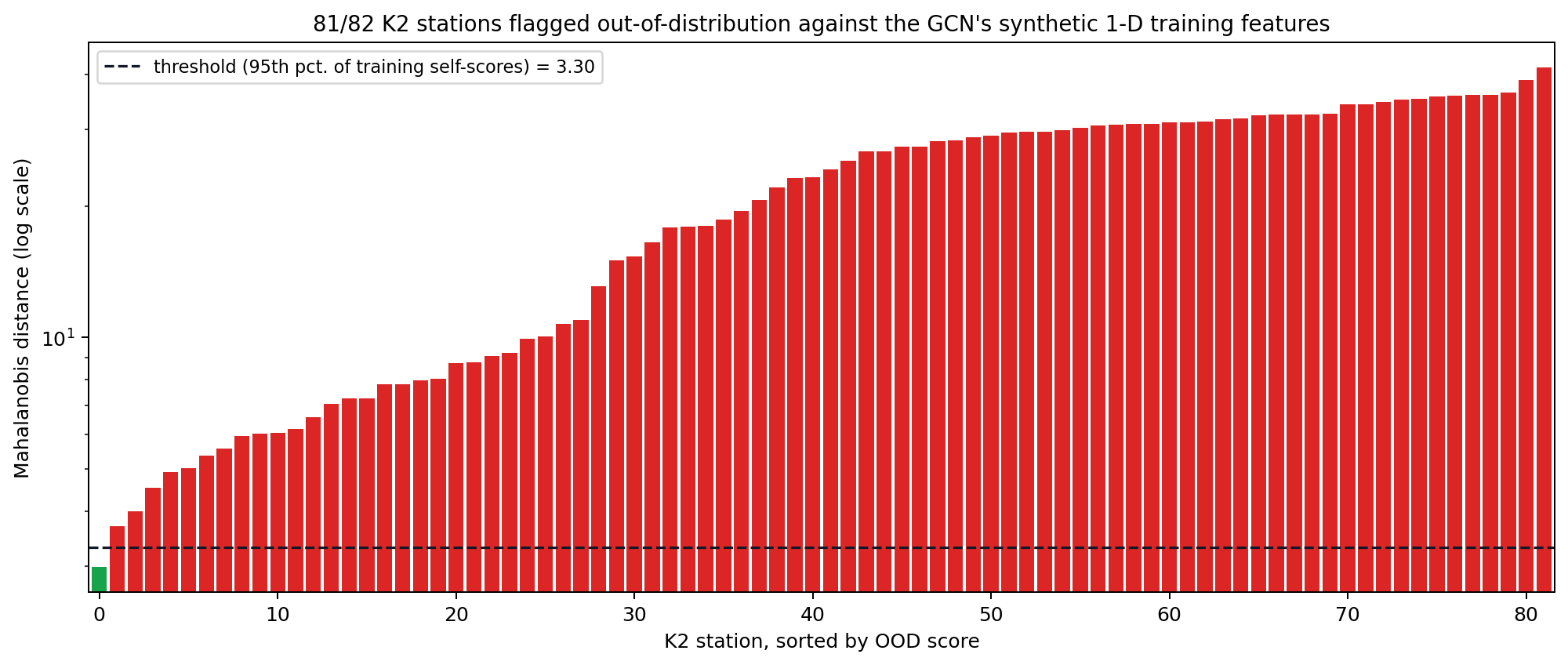
Every K2 station’s Mahalanobis distance from the GCN’s training-feature distribution, sorted, against the threshold flag_out_of_distribution() derived from the training set’s own self-scores.

Eighty-one of eighty-two stations exceed a threshold set from the training data’s own internal spread — only Z2HX051, the station sitting at the profile’s topographic high point, scores inside it. This is the quantitative version of the audit’s opening finding: a survey that is 89.8% classified 3-D, with an 84° strike disagreement between stations, does not resemble a population of independent 1-D layered soundings, which is precisely what Inv3DAgent’s training data is built from. The OOD screen would have flagged this before a single figure was drawn, using nothing but the observed data and the training configuration — no synthetic truth, no field ground truth, and no dependence on whether the final prediction happened to look plausible.

18.14.10. Recommended Decision

Three real, independently obtained pieces of evidence agree with each other on K2: the dimensionality audit (89.8% 3-D, 84° strike spread), the forward-modelled RMS (8.02 log₁₀ decades on the GCN path versus a physically plausible range on the Maxwell-based path), and the out-of-distribution screen (81 of 82 stations flagged). None of them required the field truth K2 does not have. Four conclusions carry over directly to your own corrected EDI directory:

• Audit before inverting. audit_survey’s dimensionality, strike, frequency-grid, and station-spacing checks are cheap and survey-agnostic; run them first, exactly as this tutorial did, before choosing which inversion path — or whether either — is appropriate.

• Prefer the physics-grounded path when the survey allows it. physics="mt2d"’s Maxwell-solved training data degraded gracefully here (a demonstration-scale recovery failure, but physically sensible output); the tiled-1-D GCN path degraded catastrophically on the same survey’s real strike complexity. Neither result should be trusted at this training scale, but they are not equally wrong.

• A low uncertainty is not evidence of a correct prediction. MC-dropout answered “how sure is the network of its own weights,” not “does this input resemble training data.” Pair it with an out-of-distribution screen rather than reading a small σ as a green light on its own.

• Topography here is a display correction, not new physics. Both figures drape a prediction below real station elevation; neither solver used a topographic mesh to produce it (affects_forward_physics is always False in the returned metadata). build_solver_mesh() already builds genuinely topographic meshes with air cells — it is simply not yet wired into generate_2d_maxwell_dataset or either agent, so relief this size is corrected for interpretation, not solved for.

Scaling the settings used in this tutorial up to a production run — hundreds to thousands of realizations, tens to hundreds of training epochs, and the survey’s full frequency band rather than the ten-frequency teaching grid — is exactly what Architecture roadmap’s M0–M10 milestones and Reproducible experiment configuration’s frozen, gated configuration exist to make reproducible. Once a result clears its declared acceptance criteria on held-out data, AI inversion reporting is where it turns into a package a reviewer who did not run this tutorial can actually check.

18.14.11. See Also

Condition an MT Line With Tipper and Rotation

Prepare corrected MT data before AI or classical inversion.

Prepare an Occam2D Inversion

Classical Occam2D input preparation for comparison.

Run a Pipeline From Config

Store repeatable preprocessing before the AI inversion step.

Building a Defensible 3-D AI Inversion Problem

A focused 3-D-plus-topography AI inversion walkthrough on the bundled L18PLT line.

Recovery, residual, and OOD diagnostics

Recovery, response-residual, calibration, and out-of-distribution diagnostics in full.

Domain-gap and noise simulation

Why field surveys differ from synthetic training data, and how to quantify the gap.

AI inversion

Full AI inversion user guide.