
1.6. Interpretation Plot Styles#
pycsamt.api.interp is the visual-style layer behind every
pycsamt.interp figure: hydrogeophysical colour sections, water-table
and transmissivity profiles, time-lapse and uncertainty panels, aquifer
characterization bars, and petrophysical cross-plots. It follows the same
singleton + preset + dotted-path pattern as pycsamt.api.style (see
Plot Styles), with one deliberate difference explained below: every plot
class here reads the singleton by default, with no extra step required to
make it track configuration changes.
This page uses the same five-station documentation fixture as
Interpretation workflow and
Hydrogeophysical interpretation, so the science itself
is not repeated here – see those pages for what the fixture represents and
how to build a real ResistivityModel from field
results.
>>> import numpy as np
>>> from pycsamt.interp import ResistivityModel, PetrophysicalConfig, EMHydroModel
>>> from pycsamt.interp.petrophysics import ArchieModel
>>> from pycsamt.interp import plot as iplot
>>> from pycsamt.api.interp import PYCSAMT_INTERP

>>> x_m = np.array([0.0, 250.0, 500.0, 750.0, 1000.0])
>>> z_m = np.array([5.0, 15.0, 30.0, 55.0, 90.0])
>>> rho_ohm_m = np.array([
...     [420, 380, 350, 410, 460],
...     [120,  95,  70, 110, 150],
...     [ 55,  42,  35,  48,  65],
...     [240, 190, 160, 210, 280],
...     [1800, 1500, 1200, 1650, 2100],
... ], dtype=float)
>>> resistivity_model = ResistivityModel.from_array(
...     np.log10(rho_ohm_m),
...     x_m,
...     z_m,
...     station_x=x_m,
...     station_names=["S00", "S01", "S02", "S03", "S04"],
...     method="demonstration",
... )

>>> config = PetrophysicalConfig(
...     petro=ArchieModel(m=1.8, n=2.0, a=1.0),
...     rho_w=20.0,
...     porosity_prior=0.25,
... )
>>> result = EMHydroModel(resistivity_model, config, method_tag="AMT").fit()
The singleton holds one complete InterpStyle
bundle per named preset, plus a live default slot that every plot class
actually reads from. Printing it summarises all four at once:
>>> print(PYCSAMT_INTERP)
PyCSAMTInterp — hydro-geophysical plot styles
  accessible   K='cividis'  Sw='BrBG'  wt_color='#0077bb'  fig_sec=(13.0, 5.0)
  dark         K='inferno'  Sw='cool'  wt_color='cyan'  fig_sec=(13.0, 5.0)
  default      K='viridis'  Sw='RdYlBu'  wt_color='deepskyblue'  fig_sec=(13.0, 5.0)  ← active
  publication  K='plasma'  Sw='RdBu'  wt_color='black'  fig_sec=(8.5, 3.8)
1.6.1. Section Vs. Profile Styles#
Each preset bundles two leaf dataclasses. HydroSectionStyle
governs every 2-D colour section – colourmaps per quantity (cmap_K,
cmap_Sw, cmap_phi, cmap_timelapse, cmap_spread, cmap_p50),
the water-table overlay line, station ticks, and colourbar geometry.
HydroProfileStyle governs every 1-D profile –
water-table and transmissivity colours, P10-P90 envelope shading, reference
lines, Dar-Zarrouk bar colours, and uncertainty-histogram bins. Both expose
their settings as ready-made keyword-argument dictionaries rather than raw
attributes, matching the *_kwargs() convention used throughout
pycsamt.api.style:
>>> sty = PYCSAMT_INTERP.default.section
>>> sty.cmap_for("K")
'viridis'
>>> sty.wt_kwargs()
{'color': 'deepskyblue', 'linewidth': 2.5, 'linestyle': '--', 'zorder': 5}

>>> psty = PYCSAMT_INTERP.default.profile
>>> psty.envelope_kwargs(psty.color_wt)
{'color': 'steelblue', 'alpha': 0.25}
A plot class never hard-codes these values; resolve_section_style()
and resolve_profile_style() look them up from
whatever style= argument (or None) the class was given.
1.6.2. Named Presets#
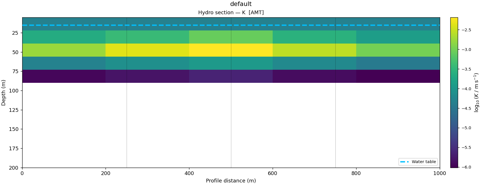
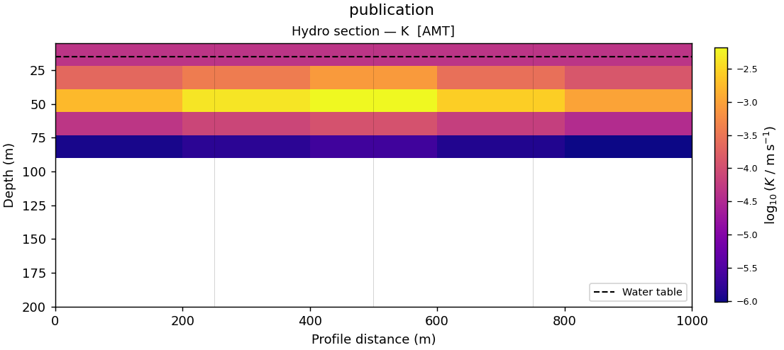
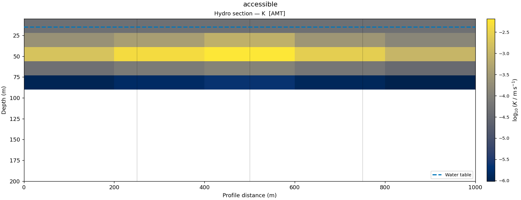
Four presets ship with the package: "default" (viridis/RdYlBu, the
package’s usual look), "publication" (compact figures, muted diverging
colourmaps, dotted zone boundaries for print), "dark" (bright cyan/white
accents and dark-friendly colourmaps such as "inferno"), and
"accessible" (the Paul Tol / IBM colorblind-safe palette). Every
pycsamt.interp.plot class defaults to style=None, which resolves
to PYCSAMT_INTERP.default – so activating a preset with
use_interp() changes every subsequent plot call
without passing style= at all:
>>> from pycsamt.api.interp import use_interp, reset_interp

>>> for preset in ["default", "publication", "dark", "accessible"]:
...     use_interp(preset)
...     fig = iplot.PlotHydroSection(result, quantity="K", depth_max=200.0).plot()
...     _ = fig.suptitle(preset)
>>> reset_interp()
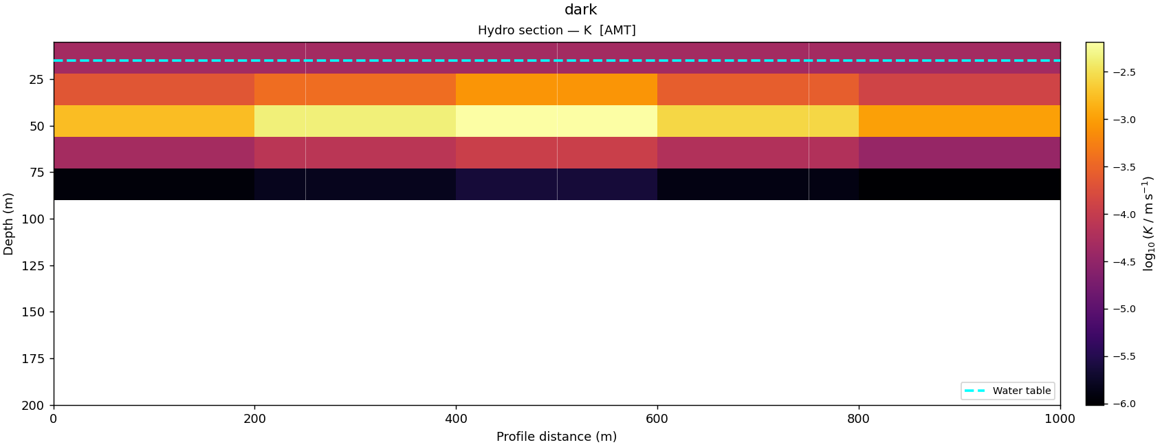
"dark" only changes colours – cyan water table, bright inferno
fill, white station ticks – it does not itself switch the figure or axes
background to a dark colour, since pycsamt.api.interp never touches
matplotlib’s rc parameters. Pair it with plt.style.use("dark_background")
(or an equivalent notebook/slide theme) for the background to actually go
dark; the preset only guarantees the drawn elements stay legible once it
does.
This is also where pycsamt.api.interp behaves differently from the
rose functions covered on Plot Styles: there, a bare
plot_phase_tensor_rose(sites) call ignores prior configure_style
edits unless style=PYCSAMT_STYLE.rose is passed explicitly. Every
pycsamt.interp.plot class instead defaults its own style
parameter to None, and None always means “read the live singleton” –
so no equivalent explicit hand-off is needed here:
>>> from pycsamt.api.interp import resolve_section_style
>>> resolve_section_style(None) is PYCSAMT_INTERP.default.section
True
>>> use_interp("dark")
>>> resolve_section_style(None).cmap_K
'inferno'
>>> reset_interp()
1.6.3. Water-Table Profile Styling#
PlotWaterTableProfile reads
HydroProfileStyle for its two panels –
water-table depth and Transmissivity:
>>> use_interp("default")
>>> fig_a = iplot.PlotWaterTableProfile(result).plot()

>>> use_interp("accessible")
>>> fig_b = iplot.PlotWaterTableProfile(result).plot()
>>> reset_interp()
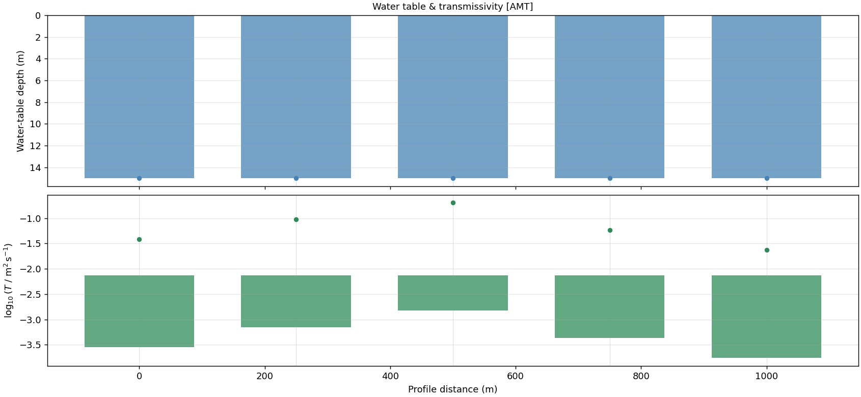
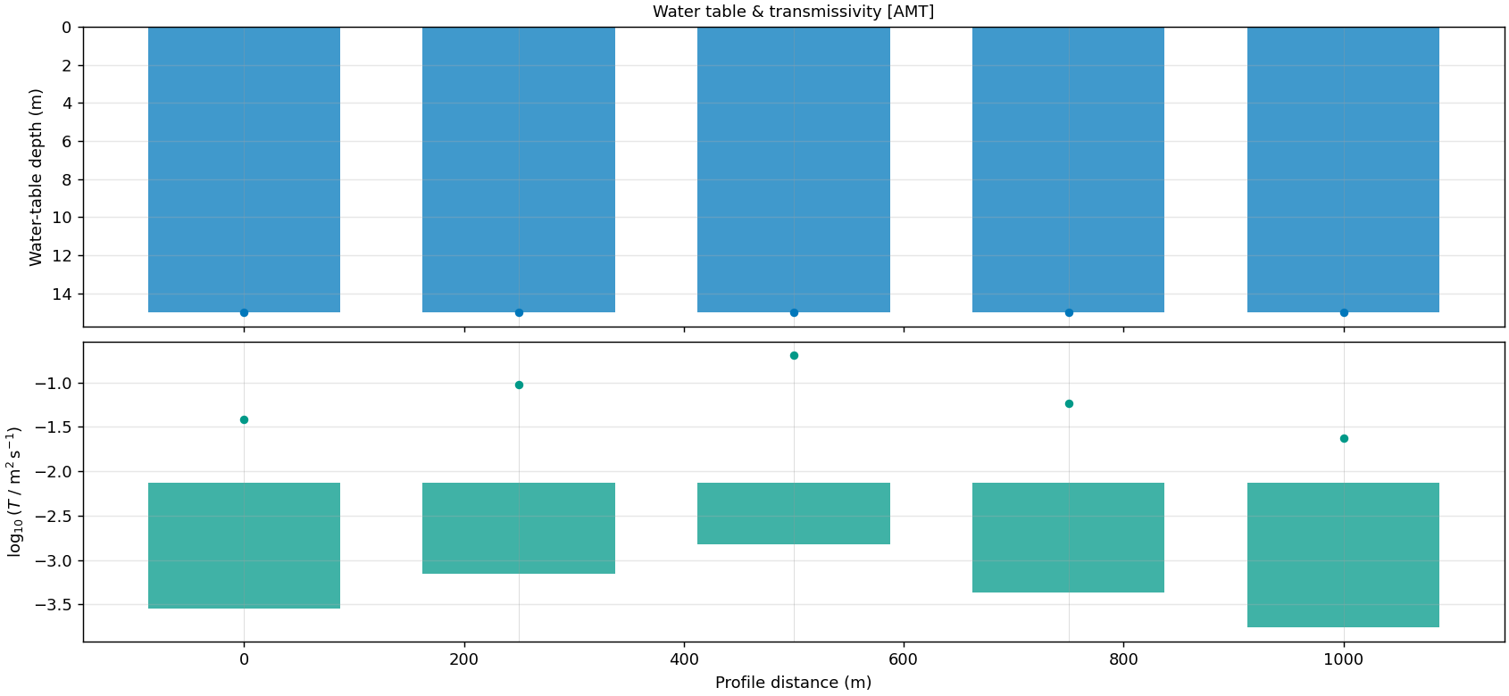
The difference is deliberately subtle here – "default"’s steelblue and
seagreen versus "accessible"’s #0077bb and #009988 – both were
chosen to already be distinguishable for the most common forms of colour
vision deficiency; the accessible preset instead guarantees it against a
wider range of viewing conditions and grayscale reproduction, not by making
the two panels look dramatically different from each other.
1.6.4. Configuring And Sharing Styles#
The same three entry points from Plot Styles apply here:
configure_interp() for dotted-path edits to the
active default bundle, PYCSAMT_INTERP.context()
for a temporary change scoped to one block, and passing a style object
directly as style= to override a single plot call without touching the
singleton at all:
>>> from pycsamt.api.interp import configure_interp

>>> configure_interp(section__cmap_K="plasma", section__wt_color="white")
>>> PYCSAMT_INTERP.default.section.cmap_K, PYCSAMT_INTERP.default.section.wt_color
('plasma', 'white')
>>> reset_interp()

>>> with PYCSAMT_INTERP.context("publication", section__wt_lw=0.8):
...     PYCSAMT_INTERP.default.section.cmap_K, PYCSAMT_INTERP.default.section.wt_lw
('plasma', 0.8)
>>> PYCSAMT_INTERP.default.section.cmap_K, PYCSAMT_INTERP.default.section.wt_lw
('viridis', 2.5)
Unlike configure_interp, which edits the live default bundle in
place, PYCSAMT_INTERP.dark (and the other three named presets) are
themselves ordinary InterpStyle instances –
copy() one and pass it as style=
to affect a single figure without calling use_interp()
at all:
>>> custom = PYCSAMT_INTERP.dark.copy()
>>> fig = iplot.PlotHydroSection(result, quantity="K", style=custom).plot()
>>> PYCSAMT_INTERP.default.section.cmap_K
'viridis'
The singleton’s own default bundle above is untouched by the explicit
style=custom call – exactly the override precedence used across every
pycsamt.api family (see API configuration).
1.6.5. Next Steps#
API configuration for how the interpretation family fits alongside every other
pycsamt.apiconfiguration family.Interpretation workflow for building a real
ResistivityModelfrom Occam2D, ModEM, or AI inversion results.Hydrogeophysical interpretation for the petrophysical models and deterministic transform behind
result– Archie’s law, Waxman-Smits, and the two-pass water-table algorithm.Uncertainty and validation for the uncertainty section and profile classes that also read
HydroSectionStyleandHydroProfileStyle.Plot Styles for the equivalent preset system used by
pycsamt.emtoolsfigures.