
8.1. Interpretation workflow#
This guide explains how to turn a reviewed electromagnetic inversion model
into a geological interpretation with pycsamt.interp. The workflow is
independent of the inversion engine: an Occam2D result, an AI-derived section,
or a generic array enters the same interpretation layer after conversion to a
pycsamt.interp.ResistivityModel.
Interpretation is not another inversion step. Inversion estimates a resistivity distribution that fits the observations under a chosen physical model and regularization. Interpretation assigns geological or hydrogeological meaning to that distribution by combining it with boreholes, field observations, prior knowledge, and uncertainty. A conductive zone can represent clay, saline water, mineralization, or several interacting effects; resistivity alone does not select one explanation.
Before you begin
Do not interpret an inversion merely because it completed successfully. Review data QC, dimensionality, static shift, error floors, convergence, residual patterns, model resolution, and sensitivity first. Preserve the original inversion result and its configuration as immutable provenance.
8.1.1. Workflow at a glance#
The recommended sequence is:
define the interpretation question and acceptable evidence;
collect the inversion result and independent constraints;
normalize the result as a
ResistivityModel;validate coordinates, depth convention, shape, units, and coverage;
preserve an unmodified calculated resistivity model;
load borehole information where it exists;
calibrate and classify the model, or classify from the rock database only;
compare the CRM and calibrated new model, including their misfit;
review station logs and spatial continuity against independent evidence;
document uncertainty and competing interpretations;
export review products together with parameters and provenance.
This order matters. Classification before geometry and unit checks can produce plausible-looking but meaningless layers. Export before scientific review can turn preliminary assumptions into apparently authoritative deliverables.
8.1.2. 1. Define the interpretation question#
Begin with a specific decision rather than a request to “interpret the section.” Examples include:
identify intervals that may correspond to weathered or fractured basement;
trace a conductive unit between boreholes;
rank locations for follow-up drilling;
test whether a resistive body is consistent with mapped geology;
prepare a calibrated resistivity section for hydrogeophysical analysis.
Record the target, expected depth range, required spatial resolution, and the evidence needed to accept or reject an interpretation. Also record known ambiguities. This prevents a later visual anomaly from silently redefining the project objective.
8.1.3. 2. Assemble the evidence package#
At minimum, retain:
the final inversion model and its mesh;
station positions and names;
observed and predicted responses;
RMS history and station/frequency residuals;
inversion configuration, error floors, regularization, and starting model;
QC and correction records, including static-shift factors;
surface geology, topography, boreholes, wells, and laboratory measurements;
coordinate reference system and profile-origin information.
Independent evidence has a different role from inversion input. A borehole used to calibrate lithology is a constraint; another borehole withheld from calibration can provide validation. Label these roles before fitting so the same observation is not counted as both training evidence and independent confirmation.
8.1.4. 3. Normalize the inversion model#
All interpretation workflows use
pycsamt.interp.ResistivityModel. Its grid follows these conventions:
x_centersis a one-dimensional array of horizontal cell centers in metres along the profile;z_centersis a one-dimensional array of depth centers in metres, positive downward;rho_2dhas shape(n_z, n_x);rho_2dcontains \(\log_{10}(\rho)\) where linear resistivity \(\rho\) is expressed in ohm metres;station_xuses the same profile origin and units asx_centers;station_namesandstation_xhave the same length.
8.1.4.1. Occam2D results#
Use the dedicated adapter when the loaded Occam2D result contains its mesh and resistivity grid:
from pycsamt.interp import ResistivityModel

model = ResistivityModel.from_occam2d(result)
The adapter obtains cell centers from mesh nodes, copies the model grid, and
preserves station offsets, station names, method name, and final RMS. It raises
ValueError when the result has no usable mesh or rho_2d grid.
8.1.4.2. Generic, AI, and converted results#
Use from_array() when arrays have
already been extracted from another backend:
import numpy as np
from pycsamt.interp import ResistivityModel

model = ResistivityModel.from_array(
    rho_2d=np.log10(rho_ohm_m),
    x_centers=x_m,
    z_centers=depth_m,
    station_x=station_offsets_m,
    station_names=station_names,
    method="modem",
    rms=1.18,
)
The five-station documentation fixture used throughout this guide builds the same way, from a plain linear-resistivity array:
>>> import numpy as np
>>> from pycsamt.interp import ResistivityModel

>>> x_m = np.array([0.0, 250.0, 500.0, 750.0, 1000.0])
>>> z_m = np.array([5.0, 15.0, 30.0, 55.0, 90.0])
>>> rho_ohm_m = np.array([
...     [420, 380, 350, 410, 460],
...     [120,  95,  70, 110, 150],
...     [ 55,  42,  35,  48,  65],
...     [240, 190, 160, 210, 280],
...     [1800, 1500, 1200, 1650, 2100],
... ], dtype=float)
>>> model = ResistivityModel.from_array(
...     np.log10(rho_ohm_m),
...     x_m,
...     z_m,
...     station_x=x_m,
...     station_names=["S00", "S01", "S02", "S03", "S04"],
...     method="demonstration",
... )
>>> model.rho_2d.shape
(5, 5)
If station_x is omitted it defaults to every horizontal cell center. If
station_names is omitted, names such as S000 are generated.
Warning
Do not pass linear resistivity to rho_2d. Convert it with
np.log10(rho_ohm_m). Conversely, do not apply np.log10 again when
the backend already stores log10 resistivity.
8.1.5. 4. Audit the normalized model#
Run explicit checks before geological classification:
>>> import numpy as np

>>> assert model.rho_2d.shape == (
...     len(model.z_centers), len(model.x_centers)
... )
>>> assert np.all(np.isfinite(model.x_centers))
>>> assert np.all(np.isfinite(model.z_centers))
>>> assert np.all(np.diff(model.x_centers) > 0)
>>> assert np.all(np.diff(model.z_centers) > 0)
>>> assert len(model.station_x) == len(model.station_names)

>>> finite = np.isfinite(model.rho_2d)
>>> if not finite.any():
...     raise ValueError("The interpretation grid contains no finite values.")

>>> rho_linear = 10.0 ** model.rho_2d[finite]
>>> print("Resistivity range:", rho_linear.min(), rho_linear.max(), "ohm m")
Resistivity range: 35.0 2099.999999999999 ohm m
>>> print("Profile length:", model.profile_length, "m")
Profile length: 1000.0 m
Also verify these questions manually:
Does profile distance increase in the expected field direction?
Is depth positive downward and referenced to surface rather than elevation?
Are station offsets in metres, not station indices or geographic degrees?
Does the interpreted depth remain inside the model’s supported depth range?
Are air, seawater, topography, padding, and inactive cells excluded or clearly identified?
Are extreme values physical, clipped bounds, or numerical placeholders?
Inspect individual columns when a section-wide pattern looks suspicious:
>>> rho_s17_log10 = model.station_column("S17")
>>> rho_at_1050_m = model.column_nearest(1050.0)
These methods return copies, so exploratory edits do not alter the source model. On the fixture, the middle station’s column is:
>>> np.round(model.station_column("S02"), 3)
array([2.544, 1.845, 1.544, 2.204, 3.079])
8.1.6. 5. Preserve the calculated resistivity model#
The inversion-derived model is the calculated resistivity model (CRM). Keep it unchanged. Calibration creates a separate model so that geological changes remain measurable and reversible.
A useful project layout is:
interpretation_project/
├── inversion/          # original model, responses, config, logs
├── constraints/        # boreholes and field observations
├── configuration/      # interpretation parameters and rock database
├── review/             # CRM/NM comparisons and validation notes
└── deliverables/       # approved tables, logs, figures, and exports
Never overwrite the original grid with interpreted lithologies. Resistivity, calibrated resistivity, lithology, and confidence are different products and should remain distinguishable.
8.1.7. 6. Load borehole constraints#
A pycsamt.interp.Borehole stores named depth intervals at a profile
position. Each interval may contain a lithology and an optional true
resistivity (TRES) in linear ohm metres.
8.1.7.1. CSV input#
The default CSV columns are top, bottom, lithology, and optional
resistivity:
top,bottom,lithology,resistivity
0,8,lateritic soil,450
8,31,clayey sand,42
31,67,weathered granite,185
67,120,fresh granite,3200
Load the file and give the borehole a position in the same profile coordinate system as the model:
from pycsamt.interp import Borehole

bh = Borehole.from_csv(
    "constraints/BH01.csv",
    name="BH01",
    x=1050.0,
    collar_elevation=238.4,
)
Loading the BH01.csv fixture shown above at x=500.0 (the middle
station, matching the profile position used throughout this guide) gives:
>>> bh = Borehole.from_csv(
...     "constraints/BH01.csv", name="BH01", x=500.0
... )
>>> bh
Borehole('BH01', x=500.0 m, 4 intervals, depth=120.0 m)
Custom column names can be supplied with top_col, bottom_col,
lithology_col, and resistivity_col. LAS 2.0 input is available through
pycsamt.interp.Borehole.from_las().
Before calibration, confirm that intervals do not overlap unexpectedly, each bottom is deeper than its top, units are metres, resistivity is linear, and the borehole’s profile position is correct. A geographically close borehole may still be inappropriate if it lies across a major structural boundary.
8.1.8. 7. Calibrate and classify#
pycsamt.interp.ModelCalibrator builds a calibrated new model (NM).
Where a nearby borehole has TRES values, cells within the fractional tolerance
ptol can be softly matched to those values. Remaining cells are assigned
using the nearest entry in the rock database in log-resistivity space.
from pycsamt.interp import ModelCalibrator

calibrator = ModelCalibrator(
    ptol=0.10,
    max_borehole_distance=500.0,
    verbose=True,
).fit(model, [bh])

calibrated_model = calibrator.calibrated_model()
misfit = calibrator.misfit_map()
logs = calibrator.stratigraphic_logs(
    model="nm",
    merge_tolerance=0.20,
)
Fitting the fixture model against BH01 (max_borehole_distance=400.0)
prints a verbose summary and reports the mean misfit:
>>> calibrator = ModelCalibrator(
...     ptol=0.10, max_borehole_distance=400.0, verbose=True,
... ).fit(model, [bh])
  ModelCalibrator: fitted 5 columns, 1 borehole(s), mean misfit G = 8.51 %
The main parameters require geological judgment:
ptolFractional CRM-to-TRES tolerance. A larger value accepts more soft replacements but does not make the evidence more certain.
max_borehole_distanceMaximum along-profile distance over which a borehole can constrain a model column. Set it according to structural continuity and station spacing, not merely to ensure every column receives a borehole constraint.
merge_toleranceLog-space tolerance used when adjacent classified cells are merged into layers. Excessive merging can hide thin units; insufficient merging can turn inversion discretization into artificial stratigraphic detail.
Calibration without boreholes is permitted:
calibrator = ModelCalibrator(verbose=False).fit(model)
logs = calibrator.stratigraphic_logs()
In that case every cell is classified from the rock database. Describe the result as a resistivity-based pseudo-stratigraphy, not as borehole-validated geology.
8.1.9. 8. Compare CRM and NM#
Calibration must be reviewed, not simply accepted. The misfit map reports the change between the calculated and calibrated models. Low change can indicate agreement; high change identifies areas where interpretation depends strongly on calibration or database assignment.
>>> import numpy as np

>>> misfit = calibrator.misfit_map()
>>> print("Mean calibration change (%):", np.nanmean(misfit))
Mean calibration change (%): 8.511650542895473
>>> print("Maximum calibration change (%):", np.nanmax(misfit))
Maximum calibration change (%): 12.409715335169182
Per-column, the fixture’s five stations were corrected by very different
amounts, because the borehole constrains the columns nearest x=500 most
strongly:
>>> np.round(misfit[0, :], 3)
array([ 3.572, 11.045, 12.41 , 12.186,  3.347])
Plot the original model, calibrated model, and misfit together:
>>> from pycsamt.interp import plot as iplot

>>> fig = iplot.PlotCalibratedModel(
...     model,
...     calibrator.calibrated_model(),
...     calibrator.misfit_map(),
... ).plot()
>>> fig.savefig("review/crm_nm_misfit.png", dpi=200, bbox_inches="tight")
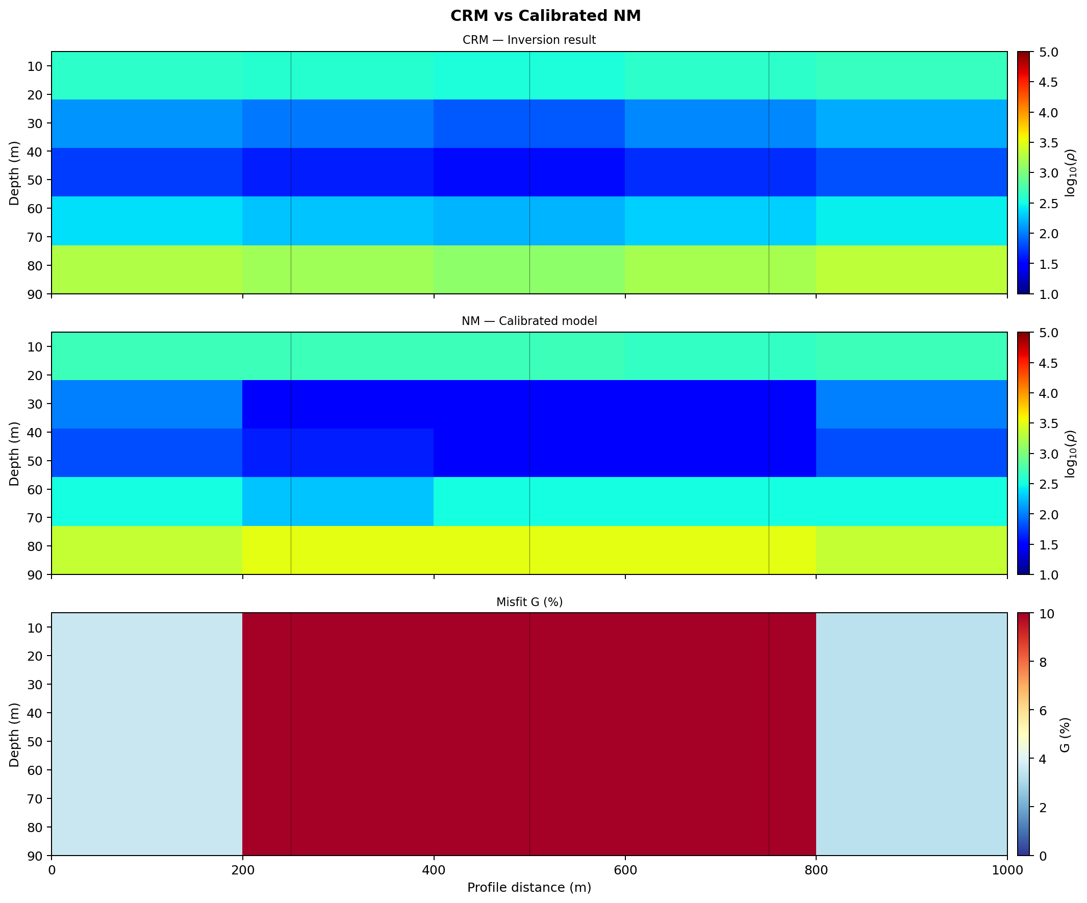
CRM (top), calibrated NM (middle), and misfit G (%) (bottom) for the
documentation fixture, produced by PlotCalibratedModel.#
Investigate broad high-misfit regions, abrupt changes at the borehole influence limit, classifications that contradict field geology, and thin alternating layers that follow mesh cells. A calibrated model is not automatically more correct than the inversion model; it is a model conditioned by additional assumptions and evidence.
8.1.10. 9. Review stratigraphic logs#
stratigraphic_logs() returns one
pycsamt.interp.StratigraphicLog per station. Compare both calibrated
and original classifications when assessing the influence of calibration:
>>> logs_nm = calibrator.stratigraphic_logs(model="nm")
>>> logs_crm = calibrator.stratigraphic_logs(model="crm")

>>> target = logs_nm[2]
>>> target.to_dict()
{'station_name': 'S02', 'station_x': 500.0, 'layers': [
 {'top': 0.0, 'bottom': 10.0, 'rho_log10': 2.6989700043360187, 'lithology': 'Sandstone'},
 {'top': 7.5, 'bottom': 42.5, 'rho_log10': 1.5, 'lithology': 'Aquifer'},
 {'top': 37.5, 'bottom': 72.5, 'rho_log10': 2.5, 'lithology': 'Granite (weathered)'},
 {'top': 72.5, 'bottom': 107.5, 'rho_log10': 3.5, 'lithology': 'Dolomite'}]}

>>> fig = iplot.PlotStratigraphicLog(target).plot()
>>> fig.savefig("review/first_station_log.png", dpi=200, bbox_inches="tight")
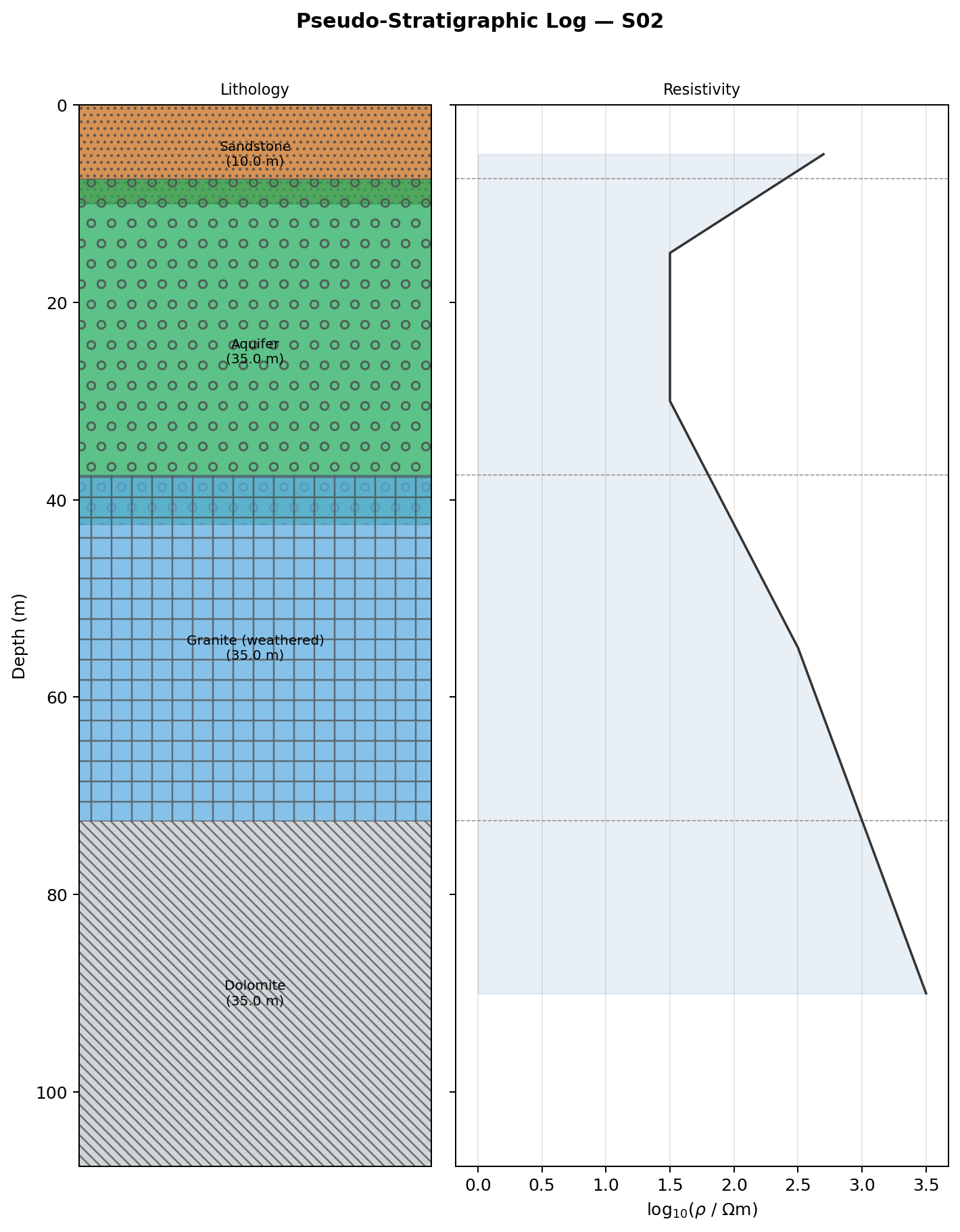
Two-panel log for station S02 from
PlotStratigraphicLog: lithology blocks on
the left, the log10-resistivity depth curve on the right.#
Layer boundaries come from midpoints between adjacent depth cells, so on an
irregular vertical mesh (this fixture uses 10, 15, 25, and 35 m spacing)
consecutive un-merged layers can report overlapping top/bottom values,
as in the Sandstone/Aquifer pair above. Treat layer boundaries as
approximate cell-edge estimates rather than exact geological contacts.
Review logs as a connected profile, not as isolated columns. Ask whether layer boundaries have geologically credible continuity, whether apparent offsets align with known structures, and whether detail exceeds the inversion’s resolution. Agreement between neighboring columns is not independent validation when regularization already enforces smoothness.
8.1.11. 10. Validate with withheld evidence#
Where possible, withhold some boreholes or observations from calibration and use them only for validation. Compare predicted boundaries and lithologies at their positions with the observed intervals. Record mismatches as well as matches.
A useful validation table contains:
observation identifier and profile position;
whether it was used for calibration;
observed interval and predicted interval;
boundary-depth difference;
lithology agreement or plausible alternatives;
local model resolution and data coverage;
reviewer decision and explanation.
Do not tune parameters repeatedly against the withheld data and continue to call it independent validation. Once used for tuning, it becomes calibration evidence and a new validation set is required.
8.1.12. 11. State uncertainty and alternatives#
Every final interpretation should distinguish at least:
data uncertainty — noise, gaps, source effects, and processing choices;
inversion uncertainty — non-uniqueness, regularization, starting model, dimensionality, and limited depth sensitivity;
petrophysical ambiguity — overlapping resistivity ranges among rocks, fluids, porosity states, alteration, and saturation;
calibration uncertainty — borehole distance, sampling quality, scale mismatch, and TRES measurement conditions;
interpretive uncertainty — assumptions used to connect electrical units to geological units.
Use confidence categories only when their criteria are written down. For example, a high-confidence boundary might require borehole control, adequate model sensitivity, agreement across inversion scenarios, and spatial continuity. Color choice or visual sharpness is not a confidence measure.
8.1.13. 12. Export reviewable products#
The interpretation export module writes station logs to common formats:
>>> from pathlib import Path
>>> from pycsamt.interp import export

>>> out = Path("deliverables")
>>> export.to_csv(logs_nm, out / "station_logs.csv")
>>> export.to_oasis_montaj_xyz(logs_nm, out / "profile.xyz")
>>> export.to_las(logs_nm[0], out / "S000.las")
>>> export.to_vtk(calibrated_model, out / "calibrated_model.vtk")
CSV is useful for auditing and downstream analysis. Oasis Montaj XYZ supports profile exchange. LAS writes a single station log. VTK carries the calibrated resistivity grid into compatible scientific viewers. See Export and reporting for the field-by-field format documentation and captured file contents for each of these exporters.
Exports are not a substitute for provenance. Accompany them with the input model identifier, coordinate reference, software version, rock database, calibration parameters, boreholes used, validation results, limitations, and the date and author of the interpretation.
8.1.14. Complete minimal example#
The following example demonstrates the complete mechanics using the small
synthetic log-resistivity grid and BH01 borehole used throughout this
guide. It was run against a real pycsamt.interp install to produce the
values shown; replace the arrays and borehole path with reviewed project
data.
>>> from pathlib import Path
>>> import numpy as np

>>> from pycsamt.interp import (
...     Borehole,
...     ModelCalibrator,
...     ResistivityModel,
...     export,
...     plot as iplot,
... )

>>> # Grid convention: rows are depths, columns are profile positions.
>>> x_m = np.array([0.0, 250.0, 500.0, 750.0, 1000.0])
>>> z_m = np.array([5.0, 15.0, 30.0, 55.0, 90.0])
>>> rho_ohm_m = np.array([
...     [420, 380, 350, 410, 460],
...     [120,  95,  70, 110, 150],
...     [ 55,  42,  35,  48,  65],
...     [240, 190, 160, 210, 280],
...     [1800, 1500, 1200, 1650, 2100],
... ], dtype=float)

>>> model = ResistivityModel.from_array(
...     np.log10(rho_ohm_m),
...     x_m,
...     z_m,
...     station_x=x_m,
...     station_names=["S00", "S01", "S02", "S03", "S04"],
...     method="demonstration",
... )

>>> bh = Borehole.from_csv(
...     "constraints/BH01.csv",
...     name="BH01",
...     x=500.0,
... )

>>> calibrator = ModelCalibrator(
...     ptol=0.10,
...     max_borehole_distance=400.0,
...     verbose=True,
... ).fit(model, [bh])
  ModelCalibrator: fitted 5 columns, 1 borehole(s), mean misfit G = 8.51 %

>>> nm = calibrator.calibrated_model()
>>> logs = calibrator.stratigraphic_logs(merge_tolerance=0.20)

>>> out = Path("deliverables")
>>> p_csv = export.to_csv(logs, out / "station_logs.csv")
>>> p_xyz = export.to_oasis_montaj_xyz(logs, out / "profile.xyz")
>>> p_vtk = export.to_vtk(nm, out / "calibrated_model.vtk")
>>> print(p_csv.as_posix())
deliverables/station_logs.csv
>>> print(p_xyz.as_posix())
deliverables/profile.xyz
>>> print(p_vtk.as_posix())
deliverables/calibrated_model.vtk

>>> fig = iplot.PlotCalibratedModel(
...     model, nm, calibrator.misfit_map()
... ).plot()
>>> fig.savefig(out / "calibration_review.png", dpi=200,
...             bbox_inches="tight")
Each exporter returns the pathlib.Path it wrote. Print
.as_posix() rather than the path itself when logging it for a manifest –
plain str()/print() renders native separators, so the same call
prints with backslashes on Windows and forward slashes on Linux or macOS.
8.1.15. Interpretation review checklist#
Before approving deliverables, confirm:
Check |
Evidence to retain |
|---|---|
Scientific question is explicit |
Target, depth range, decision, and acceptance criteria. |
Inversion is reviewable |
Configuration, convergence, residuals, QC, and sensitivity evidence. |
Geometry and units are correct |
Coordinate reference, profile origin, metres, positive-down depth, and log10 resistivity confirmation. |
CRM is preserved |
Immutable original grid and a separately identified calibrated model. |
Constraints are traceable |
Borehole sources, positions, intervals, TRES units, and calibration or validation role. |
Calibration is justified |
|
Alternatives are discussed |
Plausible competing lithologies or fluid/porosity explanations. |
Confidence is evidence-based |
Written criteria linked to resolution, calibration, and validation. |
Exports carry provenance |
Software version, inputs, parameters, limitations, author, and date. |
8.1.16. Common mistakes#
Avoid these recurring interpretation errors:
treating a smooth inversion boundary as an exact geological contact;
interpreting padding, inactive cells, or poorly sensitive depth ranges;
confusing log10 resistivity with linear ohm metres;
using geographic coordinates as profile offsets without projection;
extending a borehole constraint across an unjustified structural distance;
presenting database-only classification as ground-truthed stratigraphy;
hiding the difference between the CRM and calibrated model;
selecting only scenarios that support the preferred geological story;
reporting high numerical precision unsupported by model resolution;
exporting figures without coordinate, unit, method, or uncertainty labels.
8.1.17. Next steps#
Continue with:
Hydrogeophysical interpretation for quantitative hydrogeological transforms;
Uncertainty and validation for calibration and interpretation uncertainty;
Export and reporting for deliverable and provenance guidance;
Inversion for inversion preparation and diagnostics;
Map Tools for station maps, profiles, and spatial context.