6.2.8. MARE2DEM

pycsamt.models.mare2dem provides the pyCSAMT integration layer for MARE2DEM, a 2.5-D finite-element electromagnetic modelling and inversion code. MARE2DEM supports magnetotelluric (MT) and controlled-source electromagnetic (CSEM) workflows, adaptive triangular meshes, topography, and MPI execution.

pyCSAMT does not vendor the compiled MARE2DEM executable. Instead, it provides the tools needed to manage a MARE2DEM project around that executable:

• configuration templates for source, binary, MPI, and file-name settings;

• source download/build/location helpers;

• native .emdata, .resistivity, .poly, .settings, log, group RMS, and data-group readers/writers;

• survey builders for MT and CSEM synthetic or prepared data files;

• ZMM-to-MARE2DEM MT data conversion;

• geometry utilities for topography, UTM conversion, profile projection, polygon simplification, triangle-region assignment, and area-of-interest estimation;

• input builders, runners, result loaders, plotting helpers, model-difference utilities, merge tools, and synthetic-noise helpers.

This page is a practical guide to those pieces. It focuses on how a user should prepare, run, inspect, and archive a MARE2DEM project from pyCSAMT.

6.2.8.1. When To Use MARE2DEM

Use the MARE2DEM integration when a project needs a native 2.5-D finite-element workflow rather than a pyCSAMT built-in inversion. Common reasons include:

• a survey geometry that is naturally profile-based but not adequately treated by a simple 1-D or 2-D approximation;

• MT, CSEM, or combined data that must be represented in MARE2DEM’s native .emdata format;

• topography, seafloor, receiver, or transmitter geometry that should be explicitly represented;

• adaptive triangular discretization through Triangle/PSLG .poly geometry;

• existing MARE2DEM project files that need Python-side validation, conversion, plotting, or result loading;

• an HPC workflow where native input files are prepared locally, run on a cluster, and loaded back into pyCSAMT afterward.

MARE2DEM is not the fastest path for every inversion. If you only need a high-level backend-neutral 2-D run, start with Choosing A Model Backend. MARE2DEM is most valuable when the native file set and engine-specific control are part of the scientific workflow.

6.2.8.2. Package Map

The public MARE2DEM package surface is intentionally broad. It includes low level file readers, high level lifecycle helpers, and project utilities.

Area	Main objects	Purpose
Configuration	Mare2DEMConfig	Stores source location, compiler overrides, binary/MPI settings, inversion controls, initial model value, and default file names.
Source and binary	SourceManager	Locates, downloads, builds, and reports status for the external MARE2DEM source tree and executable.
Build inputs	InputBuilder	Writes a MARE2DEM run directory from an existing .emdata file, an EMDataFile object, or MT/CSEM survey configuration objects.
Execute	Mare2DEMRunner	Builds the command line, handles MPI options, runs the executable from the working directory, and can return an InversionResult.
Load results	InversionResult, Mare2DEMLog, GroupRMSLog	Scans output directories, parses iteration logs, exposes RMS history, convergence state, final model, observed data, and response data.
Native I/O	read_emdata, write_emdata, read_resistivity, write_resistivity, read_poly, write_poly, write_settings	Reads and writes MARE2DEM-native project files.
Data management	MTSurveyConfig, CSEMSurveyConfig, make_data_file, read_zmm, make_mt_data_from_zmm, merge_data_files	Builds, converts, and merges MT/CSEM data products.
Geometry	parse_topo, lonlat_to_utm, project_onto_line, get_line_orientation, simplify_poly, get_triangle_regions	Handles topography, survey projection, coordinate conversion, polygon cleanup, and triangle-region utilities.
QC and interpretation	NoiseConfig, add_synthetic_noise, diff_resistivity, PlotConvergence, PlotSurveyLayout, plot_poly	Supports synthetic tests, model comparison, convergence review, survey layout QC, and mesh/geometry inspection.

6.2.8.3. Configuration

Mare2DEMConfig is the source-of-truth object for MARE2DEM runs. It is a plain dataclass, so it can be created in Python, written as a configuration file template, edited outside Python, and loaded again.

>>> from pycsamt.models.mare2dem import Mare2DEMConfig

>>> cfg = Mare2DEMConfig(
...     source_dir="/opt/mare2dem/source",
...     binary="MARE2DEM",
...     use_mpi=True,
...     n_procs=16,
...     mpi_command="mpirun",
...     max_iterations=120,
...     target_rms=1.0,
...     initial_rho=10.0,
...     data_file="line12.emdata",
...     resistivity_file="line12.resistivity",
...     settings_file="line12.settings",
... )

>>> cfg.to_template("runs/line12_mare2dem_v01/mare2dem.yml")
>>> loaded = Mare2DEMConfig.from_file("runs/line12_mare2dem_v01/mare2dem.yml")
>>> print(loaded.binary, loaded.max_iterations, loaded.resistivity_stem)
MARE2DEM 120 line12

The configuration groups five concerns.

Concern	Fields	Meaning
Source management	source_dir, fc_compiler, cc_compiler	Where the Fortran source lives and which compiler commands should be used when building.
Binary and MPI	binary, use_mpi, n_procs, mpi_command	How pyCSAMT should locate and launch the executable.
Inversion control	max_iterations, target_rms	Iteration limit and normalized RMS target written into the native model/settings files.
Initial model	initial_rho	Starting homogeneous half-space resistivity, in ohm metres.
File names	data_file, resistivity_file, settings_file	Native file names used by builders and runners.

The resistivity_stem property returns the stem of resistivity_file. MARE2DEM receives this stem on the command line and then derives related filenames from it. For example, line12.resistivity is passed as line12, which is exactly what loaded.resistivity_stem printed above.

6.2.8.4. Source And Binary Management

SourceManager handles the external source tree. It resolves a source directory in this order:

1. the explicit source_dir argument passed to SourceManager;

2. Mare2DEMConfig.source_dir;

3. the PYCSAMT_MARE2DEM_SOURCE environment variable;

4. the package _source/ directory when it is writable, which is common in editable development installs;

5. a platform user-data directory.

Unlike Occam2D, pyCSAMT does not bundle MARE2DEM’s Fortran source. The package _source/ directory may exist as an empty download destination, but it is not a populated source tree until SourceManager.download succeeds. There is no compiled binary to discover on a typical machine, and none is bundled for this documentation build either – the examples below load a bundled, already-finished sample run instead (see Inspect Results), the same way ModEM does for ModEM.

This is a genuinely working, tested path, not an aspirational one: a real MARE2DEM binary has been built from this exact source-management code (inside WSL2 Ubuntu with Intel’s free oneAPI toolchain) and its forward solve validated against the analytic half-space MT response to within the binary’s own ~0.2-0.8% adaptive-mesh-refinement error – see MARE2DEM for the full build transcript and Mare2DEMAdapter’s module docstring for the physics-validation account (a separate concern from building the binary: that adapter is the AI-inversion forward-solver integration in pycsamt.forward.maxwell, distinct from the classical inversion workflow this page documents, and talks to the same compiled MARE2DEM executable through its own PSLG-based mesh convention).

The complete supported build procedure, including Intel oneAPI, MKL, WSL, download behavior, and the pycsamt build wrapper, is documented at MARE2DEM. In a Linux or WSL installation that uses the standard oneAPI location, the short form is:

source /opt/intel/oneapi/setvars.sh
pycsamt build mare2dem --auto-install -y \
    --source-dir /opt/mare2dem/source

On macOS or a non-standard Linux installation, source the corresponding setvars.sh path for that oneAPI installation before running the same pycsamt build command. Choose a writable --source-dir and reuse that exact path as Mare2DEMConfig.source_dir; /opt/mare2dem/source is only an example and may require administrator-created directory permissions.

Do not run that command from native Windows PowerShell or cmd.exe; MARE2DEM cannot be compiled natively on Windows. Enter WSL first and keep the source, build, and run paths visible inside that WSL environment.

Use status before downloading or building, and again afterward to record the resolved source and executable paths:

>>> from pycsamt.models.mare2dem import Mare2DEMConfig, SourceManager

>>> cfg = Mare2DEMConfig(source_dir="/opt/mare2dem/source")
>>> source = SourceManager(config=cfg, verbose=1)

>>> source.print_status()
MARE2DEM SourceManager status
────────────────────────────────────────
  source_dir  : /opt/mare2dem/source
  downloaded  : False
  built       : False
  binary      : (not found)
  FC compiler : mpifort
  CC compiler : mpicc
  MKLROOT     : (not found — required)

When source code is not present, download can use Git or a source archive. When source code is present but the binary is missing, build compiles the external code. These direct Python calls are equivalent to the lifecycle managed by the build wrapper and are useful when a cluster needs a custom Make include file:

>>> from pycsamt.models.mare2dem import SourceManager

>>> source = SourceManager(source_dir="/opt/mare2dem/source", verbose=1)

>>> # Network access and compiler availability are environment-dependent.
>>> # source.download(method="auto")
>>> # binary = source.build(clean_first=False)
>>> # print(binary)

MARE2DEM requires an MPI Fortran/C toolchain and Intel MKL for ScaLAPACK/BLACS. Prefer Intel mpiifx/mpiicx (current oneAPI releases) or the classic mpiifort/mpiicc (older ones) with oneAPI initialized; generic mpifort/mpicc may be detected by SourceManager but do not remove the MKL requirement and are not a guarantee of a usable build. The missing MKLROOT in the status above is that prerequisite being detected before compilation. See MARE2DEM for a real, successful build transcript and the toolchain-detection bugs a real build run against a current oneAPI installation surfaced and fixed.

6.2.8.5. Binary Resolution

Mare2DEMRunner resolves the executable through:

1. Mare2DEMConfig.binary on PATH (an explicit executable path is also accepted by shutil.which);

2. <source_dir>/<binary>;

3. the platform user-data binary location.

Use runner.command as a dry-run check before launching an inversion. Note that command() formats the configured command but does not prove that the executable or MPI launcher exists. Use SourceManager.resolve_binary for the executable preflight performed by run():

>>> from pycsamt.models.mare2dem import (
...     Mare2DEMConfig,
...     Mare2DEMRunner,
...     SourceManager,
... )

>>> cfg = Mare2DEMConfig(
...     binary="MARE2DEM",
...     use_mpi=True,
...     n_procs=8,
...     mpi_command="mpirun",
...     resistivity_file="line12.resistivity",
... )

>>> runner = Mare2DEMRunner("runs/line12_mare2dem_v01/native", config=cfg)
>>> binary = SourceManager(config=cfg).resolve_binary()
>>> if binary is None:
...     raise FileNotFoundError(
...         "MARE2DEM was not built; see the MARE2DEM compilation guide"
...     )
>>> print(binary)
/opt/mare2dem/source/MARE2DEM
>>> print(runner.command("line12"))
mpirun -np 8 MARE2DEM line12

For cluster workflows, put the command string and the loaded module list in the run provenance manifest. The same native directory can then be executed by a job scheduler and loaded later with InversionResult.

6.2.8.6. Native Files

MARE2DEM projects revolve around native files. pyCSAMT treats these as first-class scientific records, not temporary build artifacts.

File	Reader/writer	Role
.emdata	read_emdata, write_emdata	Observed or synthetic MT/CSEM/DC data, receiver/transmitter metadata, UTM origin, frequencies, and data rows.
*_MARE2DEM.emdata or .resp	read_emdata	Predicted response data produced by the engine.
.resistivity	read_resistivity, write_resistivity	Resistivity parameters, free/fixed flags, bounds, prejudice values, and references to data, settings, and polygon files.
.poly	read_poly, write_poly	Triangle PSLG geometry: nodes, segments, holes, and regions.
.settings	write_settings	Parallel decomposition and inversion settings.
.emdata_group	read_data_group, write_data_group	Group definitions used for grouped RMS diagnostics.
Group RMS logs	read_group_rms_log	Per-group RMS evolution, useful for diagnosing which data families are controlling the inversion.
Iteration logs	Mare2DEMLog	Iteration number, RMS misfit, roughness, Lagrange multiplier, and convergence state.

The validation helpers classify common MARE2DEM files by filename pattern alone – unlike the Occam2D and ModEM validators, they do not need the file to exist or read its contents, so they also work as a naming-convention check before a file has been written:

>>> from pycsamt.models.mare2dem import detect_file_type, is_response_file

>>> print(detect_file_type("line12.emdata"))
Mare2DEMFileType.EMDATA
>>> print(detect_file_type("line12.resistivity"))
Mare2DEMFileType.RESISTIVITY
>>> print(is_response_file("line12_MARE2DEM.emdata"))
True

6.2.8.7. Build A Run Directory

InputBuilder writes a minimal MARE2DEM input set. It can start from an existing .emdata file, an in-memory EMDataFile, or MT/CSEM survey configuration objects. This example starts from a real bundled synthetic MT line:

>>> from pycsamt.models.mare2dem import InputBuilder, Mare2DEMConfig

>>> cfg = Mare2DEMConfig(
...     initial_rho=10.0,
...     max_iterations=120,
...     target_rms=1.0,
...     data_file="line12.emdata",
...     resistivity_file="line12.resistivity",
...     settings_file="line12.settings",
... )

>>> builder = InputBuilder(config=cfg, verbose=1)
>>> files = builder.build(
...     "data/mare2dem/demo_mt_inversion/demo_mt_synth.emdata",
...     workdir="runs/line12_mare2dem_v01/native",
... )

>>> print(files["data"].name, files["model"].name, files["settings"].name)
line12.emdata line12.resistivity line12.settings

The builder writes:

• the data file, copied or generated into the run directory;

• a homogeneous starting .resistivity file based on initial_rho;

• a .settings file.

For production inversions, the generated starting model is often only the first step. Review the .resistivity and .poly inputs before launching the external code.

6.2.8.8. Create MT Data

MTSurveyConfig and make_data_file are useful for synthetic tests or for constructing simple MT-native files from survey arrays.

>>> import numpy as np

>>> from pycsamt.models.mare2dem import MTSurveyConfig, make_data_file

>>> mt = MTSurveyConfig(
...     frequencies=np.logspace(-3, 3, 25),
...     rx_y=np.linspace(-6000.0, 6000.0, 31),
...     rx_type="land",
...     lTE=True,
...     lTM=True,
...     lTipper=False,
... )

>>> em = make_data_file(
...     "runs/line12_mare2dem_v01/native/line12_mt.emdata",
...     topo=0.0,
...     mt=mt,
... )

>>> print(em.n_data)
3100

For real MT processing, pyCSAMT also includes ZMM readers and converters (read_zmm, make_mt_data_from_zmm). No ZMM sample ships with pyCSAMT, so they are not exercised with captured output here – read_zmm(path) returns a ZMMStation with .name, .latitude/.longitude, and impedance/tipper arrays, and make_mt_data_from_zmm accepts a list of such files plus error-floor and topography options, mirroring make_data_file.

Check the generated data rows carefully. Conversion utilities help with file mechanics, but the interpreter still owns station selection, component choice, frequency band selection, and error-floor policy.

6.2.8.9. Create CSEM Data

CSEMSurveyConfig builds a controlled-source survey with transmitter and receiver layout parameters.

>>> import numpy as np

>>> from pycsamt.models.mare2dem import CSEMSurveyConfig, make_data_file

>>> csem = CSEMSurveyConfig(
...     frequencies=np.array([0.25, 0.5, 1.0, 2.0]),
...     rx_y=np.linspace(-4000.0, 4000.0, 17),
...     tx_y=np.array([-2500.0, 0.0, 2500.0]),
...     rx_type="marine",
...     tx_type="edipole",
...     lEx=True,
...     lEy=True,
...     lBx=True,
...     lBy=True,
... )

>>> em = make_data_file(
...     "runs/csem_line_v01/native/csem_line.emdata",
...     topo=-1000.0,
...     csem=csem,
... )

>>> print(em.n_data)
1632

rx_type and tx_type look like the same kind of setting but are not: rx_type is a placement mode ("land", "marine", "amphibious"), while tx_type is a dipole physics type and only understands "edipole" or "bdipole". Passing a placement word such as "marine" as tx_type does not raise an error – it is silently written to the .emdata file’s Type column as the literal string "marine", which downstream pyCSAMT code that reads that column back (for example the merge tools in Merge And Noise Utilities) treats as "bdipole", since only an exact "edipole" match counts otherwise. A towed marine CSEM transmitter is normally an electric dipole, so the correct value here is tx_type="edipole", not tx_type="marine".

For CSEM projects, geometry QC is essential. Plot receiver/transmitter locations, confirm signs and offsets, and record whether coordinates are local profile coordinates, UTM coordinates, or a transformed system – see Plotting And QC below for PlotSurveyLayout.

6.2.8.10. Merge And Noise Utilities

MARE2DEM workflows often require combining data families or creating synthetic observations from a forward response. pyCSAMT provides utilities for both. Merging a real bundled MT line with a real bundled CSEM line demonstrates a genuine joint-data use case:

>>> from pycsamt.models.mare2dem import merge_data_files

>>> merged = merge_data_files(
...     [
...         "data/mare2dem/demo_mt_inversion/demo_mt_synth.emdata",
...         "data/mare2dem/demo_csem/demo_csem.emdata",
...     ],
...     "runs/joint_v01/native/joint.emdata",
... )

>>> print(merged.n_data)
852

Synthetic noise is useful for controlled tests and algorithm validation. Setting seed makes the result reproducible – record it in the run provenance manifest alongside the noise parameters:

>>> from pycsamt.models.mare2dem import (
...     NoiseConfig,
...     add_synthetic_noise,
...     read_emdata,
...     write_emdata,
... )

>>> response = read_emdata("data/mare2dem/demo_mt_inversion/demo.6.resp")
>>> noise = NoiseConfig(
...     mt_rel_noise=0.05,
...     mt_abs_noise_tipper=0.01,
... )

>>> synthetic = add_synthetic_noise(response, noise, seed=42)
>>> write_emdata(synthetic, "runs/synthetic_v01/native/synthetic.emdata")
>>> print(synthetic.n_data, response.n_data)
572 572

Do not treat noisy synthetic data as field data. Keep synthetic sources, random seeds, and noise parameters in the provenance notes.

6.2.8.11. Geometry And Topography

The MARE2DEM integration includes geometry helpers because geometry mistakes are one of the easiest ways to produce convincing but wrong models.

Helper	Use
parse_topo, topo_depth, topo_slope	Read and interpolate topography/seafloor profiles and compute local slopes.
lonlat_to_utm, utm_to_lonlat	Convert coordinates with pyproj when available and a pure-Python WGS-84 fallback otherwise.
get_line_orientation, project_onto_line	Estimate profile orientation and project stations onto a survey line.
dp_simplify, simplify_poly	Simplify polylines and remove collinear polygon nodes.
get_intersections, do_rects_overlap	Find segment intersections with bounding-box pre-filtering.
triangle_centroids, triangle_areas, get_centroids	Compute area-weighted centroids and triangle geometry summaries.
estimate_area_of_interest	Estimate a practical modelling area from survey geometry.
get_triangle_regions	Assign finite-element regions for Triangle-based meshes.

Example profile projection:

>>> import numpy as np

>>> from pycsamt.models.mare2dem import (
...     get_line_orientation,
...     lonlat_to_utm,
...     project_onto_line,
... )

>>> lon = np.array([11.501, 11.507, 11.514])
>>> lat = np.array([3.842, 3.845, 3.849])

>>> east, north, zone, south_hemi = lonlat_to_utm(lon, lat)
>>> azimuth = get_line_orientation(north, east)
>>> cross_profile, along_profile = project_onto_line(
...     north,
...     east,
...     north[0],
...     east[0],
...     azimuth,
... )

>>> print(f"zone {zone}, southern hemisphere: {south_hemi}")
zone 32, southern hemisphere: False
>>> print(along_profile)
[   0.          744.48607367 1639.22643014]

lonlat_to_utm returns south_hemi as a plain boolean, not the "N"/ "S" letter some other UTM tools use – False here means the three points (all near latitude 3.8°) are in the northern hemisphere, matching their positive latitude.

For production documentation, include a small figure or table showing original coordinates, projected distances, and topography values. That record is often as important as the inversion result.

6.2.8.12. Grid And Mesh Utilities

The package includes helpers for constructing MARE2DEM geometry and models from gridded resistivity information. grid_to_mare2dem takes the grid as three 2-D arrays shaped like a numpy.meshgrid output – Y and Z are coordinate grids, not axis vectors, and Rho is the cell-centred resistivity on that same grid:

>>> import numpy as np

>>> from pycsamt.models.mare2dem import grid_to_mare2dem

>>> y_c = np.linspace(-2000.0, 2000.0, 20)
>>> z_c = np.linspace(50.0, 1000.0, 12)
>>> Y, Z = np.meshgrid(y_c, z_c)
>>> Rho = np.full((12, 20), 100.0)
>>> Rho[3:6, 8:12] = 10.0  # a shallow conductive block

>>> files = grid_to_mare2dem(
...     Y, Z, Rho,
...     out_dir="runs/grid_model_v01/native",
...     model_name="line12",
...     data_file="line12.emdata",
... )

>>> print(files["poly"].name, files["resistivity"].name)
line12.poly line12.0.resistivity

Always inspect the written .poly and .resistivity files before using them in an inversion – plot_poly (see Plotting And QC) is the fastest way to confirm the padding and region layout came out as expected.

6.2.8.13. Run MARE2DEM

Once native files are prepared and the executable is available, use Mare2DEMRunner to launch the run. Keep source_dir in the saved configuration pointed at the same source tree used by MARE2DEM; otherwise the runner cannot find a locally built binary that is not also on PATH.

>>> from pycsamt.models.mare2dem import (
...     Mare2DEMConfig,
...     Mare2DEMRunner,
...     SourceManager,
... )

>>> cfg = Mare2DEMConfig.from_file("runs/line12_mare2dem_v01/mare2dem.yml")
>>> runner = Mare2DEMRunner("runs/line12_mare2dem_v01/native", config=cfg, verbose=1)

>>> # Resolve the binary before submitting a long job.
>>> source = SourceManager(config=cfg)
>>> binary = source.resolve_binary()
>>> if binary is None:
...     raise FileNotFoundError(
...         "MARE2DEM was not built; see the MARE2DEM compilation guide"
...     )
>>> print(binary)
/opt/mare2dem/source/MARE2DEM

>>> # Inspect the logical command before running it.
>>> print(runner.command(cfg.resistivity_stem))
mpirun -np 16 MARE2DEM line12

command() deliberately shows cfg.binary rather than the absolute path resolved above. During execution, run() resolves that name through SourceManager and launches the resulting executable.

Run only after confirming that the resistivity stem names matching native files in runner.workdir. Pass the stem ("line12"), not a path to a file in another directory; the runner intentionally strips directory and suffix components and executes from workdir:

result = runner.run(
    cfg.resistivity_stem,
    use_mpi=True,
    n_procs=16,
    extra_args=None,
    timeout=None,
    load_result=True,
)

The run block is intentionally not a doctest: it launches an MPI inversion that may run for hours. A non-zero solver exit raises subprocess.CalledProcessError; a configured timeout raises subprocess.TimeoutExpired. With load_result=True, a successful run returns InversionResult. Set it to False when a scheduler or a later process will load the completed directory.

MARE2DEM is normally an MPI program. Before local execution, verify that cfg.mpi_command resolves in the same shell environment as Python and that cfg.n_procs is appropriate for the allocation. Do not set use_mpi=False unless the executable was specifically built for single-process operation.

For long inversions, prefer scheduler-managed execution. Build the native directory with pyCSAMT, submit the command on the cluster, then use InversionResult after the files are complete.

6.2.8.14. Inspect Results

InversionResult scans a run directory for recognized output files and exposes the main products.

None of the sections above actually launched MARE2DEM – there is no compiled binary in a documentation-build environment. From here on, the examples load a genuinely finished run instead: the bundled data/mare2dem/demo_mt_inversion sample, a real converged 6-iteration MT inversion.

>>> from pycsamt.models.mare2dem import InversionResult

>>> result = InversionResult("data/mare2dem/demo_mt_inversion")

>>> print(result.converged, result.final_rms, result.n_iterations)
True 1.002 6

result.model is populated from whichever .resistivity file the directory scan happens to encounter first – it is not guaranteed to be the highest-numbered iteration. This sample directory keeps both demo.0.resistivity (the starting half-space) and demo.6.resistivity (the converged final model), and because "demo.0" sorts before "demo.6", result.model here silently resolves to the starting model:

>>> print(result.model.resistivity_file, result.model.iteration)
demo.0.resistivity 0

Nothing raises or warns about this. When a directory holds more than one resistivity snapshot, load the specific file you actually want with read_resistivity instead of trusting result.model:

>>> from pycsamt.models.mare2dem import read_resistivity

>>> model_final = read_resistivity(
...     "data/mare2dem/demo_mt_inversion/demo.6.resistivity"
... )
>>> print(model_final.resistivity_file, model_final.num_regions)
demo.6.resistivity 6540

The log parser exposes the RMS, roughness, and Lagrange-multiplier (\(\log_{10}\mu\)) history per iteration.

>>> from pycsamt.models.mare2dem import Mare2DEMLog

>>> log = Mare2DEMLog("data/mare2dem/demo_mt_inversion/demo.logfile")

>>> print(log.final_rms, log.converged)
1.002 True
>>> print(log.rms_history())
[6.875, 3.336, 1.719, 1.074, 1.001, 1.002]
>>> print([round(rec.roughness, 3) for rec in log.iterations])
[1.407, 7.278, 20.39, 36.76, 39.39, 37.44]

Mare2DEMLog has no roughness_history() method – roughness (and rms, lambda_) live on each entry of log.iterations, a list of IterationRecord objects, one per completed iteration. The trade-off here is exactly the one the objective function implies: as RMS drops by more than 6x (6.875 to 1.001) over the first five iterations, roughness climbs nearly 28-fold (1.41 to a peak of 39.4) – the smoothest model that still fits the data is far less smooth than the uniform starting half-space, and roughness keeps climbing even in iteration 6, where RMS has already flattened.

Group RMS logs should be reviewed when the inversion combines data types, components, stations, or source groups.

>>> from pycsamt.models.mare2dem import read_group_rms_log

>>> group_log = read_group_rms_log(
...     "data/mare2dem/demo_csem_mt/demo.group_rms.log"
... )
>>> print(group_log.headers)
['Iteration', 'Total RMS', 'CSEM', 'MT']
>>> print(group_log.rms_log[-1])
[20.     0.998  0.912  1.038]

A low total RMS can hide a poor fit to one group. Inspect total RMS, group RMS, response residuals, and model roughness together – here the joint run’s total RMS (0.998) is a blend that looks slightly better than either the CSEM group (0.912) or the MT group (1.038) taken alone.

6.2.8.15. Plotting And QC

The plotting helpers are designed for quality control and interpretation. All figures below use the same converged demo_mt_inversion result loaded above, plus the bundled CSEM sample for survey-layout QC.

Plot helper	Use
PlotConvergence	RMS and convergence history from logs.
PlotSurveyLayout	Receiver/transmitter layout in map/profile coordinates.
PlotRxParams	Receiver geometry and parameter checks.
PlotTxParams	Transmitter geometry and parameter checks.
plot_poly	PSLG/.poly geometry inspection.
PlotModel	Model-section visualization support.
PlotResponse	Observed/predicted response inspection.

>>> from pycsamt.models.mare2dem import Mare2DEMLog, PlotConvergence

>>> log = Mare2DEMLog("data/mare2dem/demo_mt_inversion/demo.logfile")
>>> fig = PlotConvergence(log).plot()
>>> fig.savefig("runs/line12_mare2dem_v01/figures/convergence.png", dpi=200)

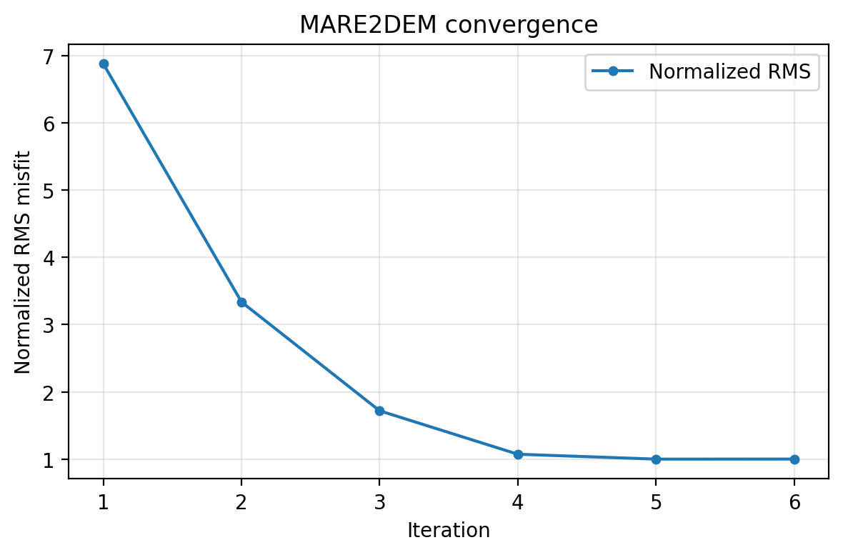
A clean, fast convergence – RMS falls from 6.9 to 1.0 in just 6 iterations and stays there. This is a useful contrast with ModEM’s bundled sample, which stalls at RMS 3.06 after 74 iterations: convergence behaviour varies enormously between real runs, which is exactly why it needs checking every time rather than assumed.

PlotModel draws a true triangulated section when Triangle’s .node/.ele mesh files are present next to the .resistivity file. This bundled sample does not include them (they are regenerated by Triangle during a run, not archived here), so PlotModel falls back to a plain histogram of every region’s resistivity – and that fallback has two rough edges worth knowing about: it labels the axis "log10 rho" while actually plotting linear values, and it does not separate free parameter regions from fixed ones such as the boundary padding cell held at \(10^{12}\,\Omega\cdot\mathrm{m}\). Filtering to free parameters and taking log10 explicitly gives a far more useful view of the same file:

>>> import numpy as np

>>> from pycsamt.models.mare2dem import read_resistivity

>>> model_final = read_resistivity(
...     "data/mare2dem/demo_mt_inversion/demo.6.resistivity"
... )
>>> rho = np.asarray(model_final.resistivity)[:, 0]
>>> free = np.asarray(model_final.free_parameter).ravel()
>>> free_rho = rho[free != 0]  # drop air/ocean/boundary regions
>>> print(free_rho.size, round(free_rho.min(), 3), round(free_rho.max(), 3))
6538 0.307 242.08

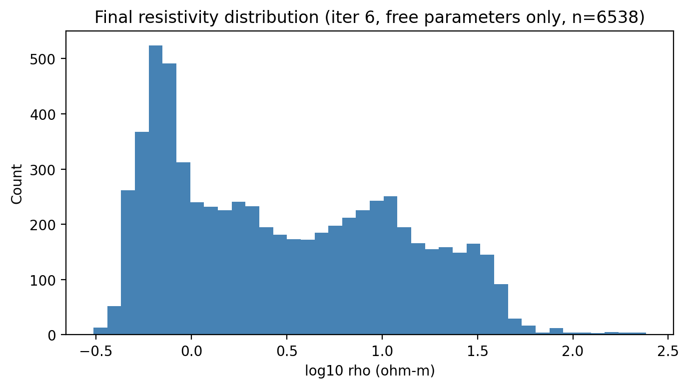
The converged model’s free-parameter resistivity is clearly bimodal: one mode around 0.6-1 ohm-m and a second, broader mode around 8-15 ohm-m, with a long tail out to 242 ohm-m. Neither mode is visible at all in the library’s default (unfiltered, linear-axis) fallback histogram, where the single \(10^{12}\) boundary region compresses everything else into one bin.

>>> from pycsamt.models.mare2dem import PlotResponse

>>> fig = PlotResponse(result).plot()
>>> fig.savefig("runs/line12_mare2dem_v01/figures/response.png", dpi=200)

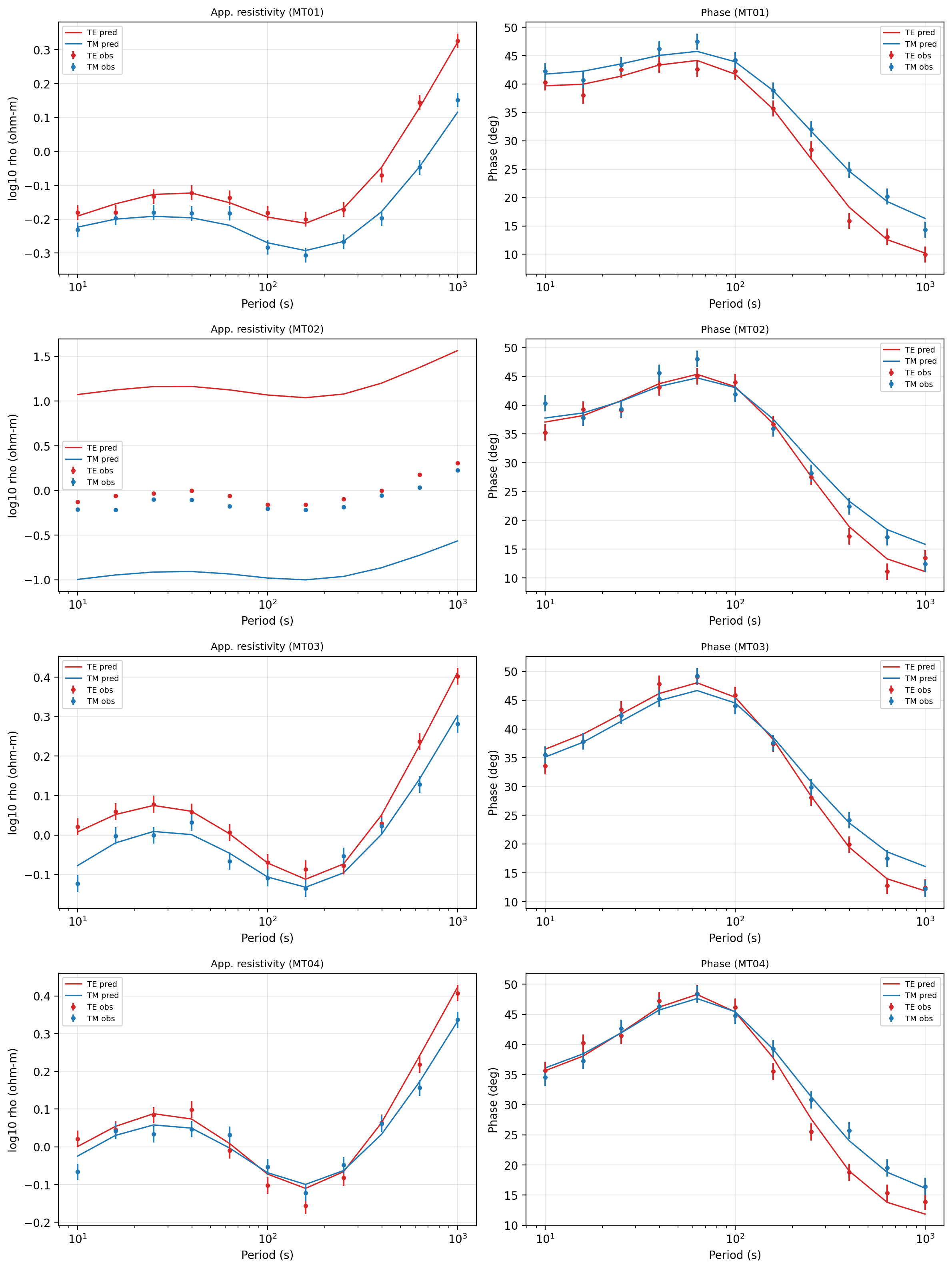
Station-level response fits for the first four MT receivers. MT01, MT03, and MT04 track the observed apparent resistivity and phase closely, but MT02’s predicted TE and TM curves sit roughly one log10 unit away from its own observations – a ten-fold resistivity mismatch at a single station, invisible in the overall RMS of 1.002. This is precisely the “low total RMS can hide a poor fit to one group” caution from Inspect Results, playing out at the station level instead of the group level.

>>> from pathlib import Path

>>> from pycsamt.models.mare2dem import PlotSurveyLayout, read_emdata

>>> em = read_emdata("data/mare2dem/demo_csem/demo_csem.emdata")
>>> fig = PlotSurveyLayout(em).plot()
>>> ax = fig.axes[0]
>>> ax.set_title(Path(em.path).name, fontsize=9)  # default title is the full path
>>> fig.savefig("runs/csem_line_v01/figures/survey_layout.png", dpi=200)

PlotSurveyLayout titles the figure with str(em.path) – the full path used to read the file, absolute if that is what was passed in. Resetting the title to just the filename keeps the figure shareable without leaking a local directory layout.

Receivers and transmitters for the bundled CSEM demo, interleaved along one straight ~26 km line. The equal-aspect map view is correct, not a rendering glitch – a genuinely linear towed/fixed CSEM deployment looks exactly this flat when Easting and Northing share a scale.

>>> from pycsamt.models.mare2dem import plot_poly

>>> ax = plot_poly(
...     "data/mare2dem/demo_mt_inversion/demo.poly",
...     savefig="runs/line12_mare2dem_v01/figures/poly.png",
...     dpi=200,
... )

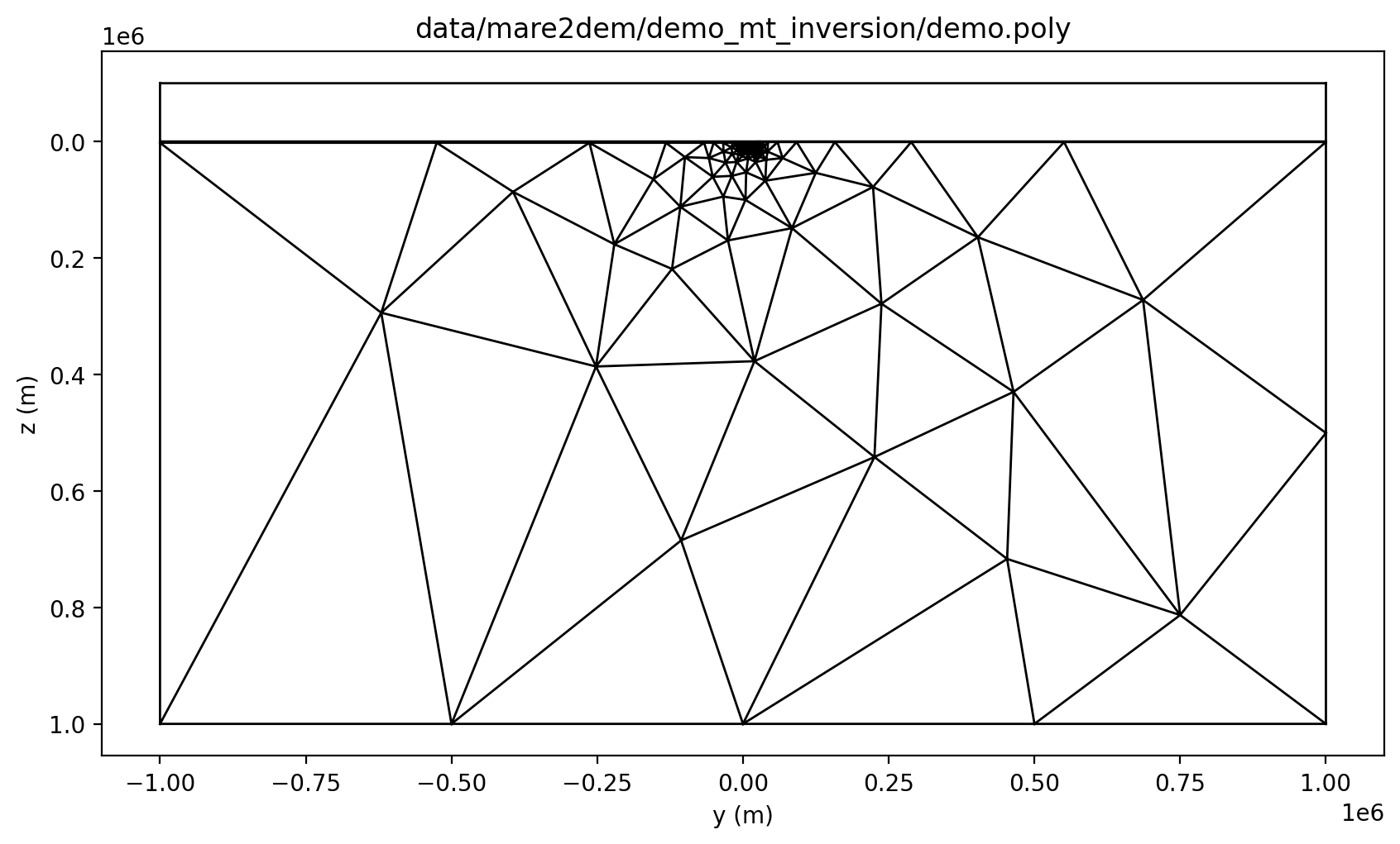
The coarse boundary PSLG behind the triangulated model – padding triangles reaching out to +-1000 km and 1000 km depth, with a dense cluster of small seed regions near \(y=0\) where the actual survey sits. Triangle refines this outline into the fine mesh MARE2DEM solves on; plot_poly shows the outline pyCSAMT wrote, before that refinement.

Before presenting a final model, review at least:

• station and transmitter geometry;

• topography or bathymetry representation;

• mesh or polygon geometry;

• RMS history and convergence status;

• group RMS history;

• observed/predicted response fits;

• model smoothness, bounds, and fixed/free parameter behavior.

6.2.8.16. Model Comparison

diff_resistivity compares two .resistivity files, typically to inspect how a model changed between iterations, parameter choices, or preprocessing decisions. Comparing the bundled sample’s starting and final models quantifies the same change Inspect Results described qualitatively:

>>> from pycsamt.models.mare2dem import diff_resistivity

>>> diff = diff_resistivity(
...     "data/mare2dem/demo_mt_inversion/demo.0.resistivity",
...     "data/mare2dem/demo_mt_inversion/demo.6.resistivity",
...     "runs/comparison_v01/demo_iter6_minus_iter0.resistivity",
... )
>>> print(diff)
ResistivityFile(num_regions=6540, anisotropy='isotropic', target_misfit=1.0)

Use model differences as diagnostics, not as standalone geological evidence. Pair them with data-fit changes and model regularization changes.

6.2.8.17. Recommended Run Layout

Keep source/build material separate from scientific run directories.

external/
  mare2dem/
    source/
    build_notes.md

runs/
  survey_alpha/
    line12_mare2dem_v01/
      mare2dem.yml
      provenance.yml
      native/
        line12.emdata
        line12.poly
        line12.resistivity
        line12.settings
        demo.logfile
        line12_MARE2DEM.emdata
        line12.group_rms.log
      qc/
        survey_layout.png
        convergence.png
        response.png
      exports/
        line12_snapshot.zip

Use versioned run names. MARE2DEM uses simple native filenames, so running several experiments in one directory can easily mix stale outputs with new inputs – and, as Inspect Results showed, can leave InversionResult loading the wrong iteration’s model without any error.

6.2.8.18. Pre-Run Checklist

Before launch:

• load Mare2DEMConfig from the edited template;

• confirm source directory and executable resolution;

• check runner.command and record it;

• confirm MPI process count and scheduler settings;

• verify that .emdata, .resistivity, .settings, and .poly files exist when required;

• inspect station, transmitter, and profile coordinates;

• inspect topography or seafloor representation;

• confirm frequency band, components, and error floors;

• confirm tx_type is a real dipole type ("edipole"/"bdipole"), not a placement word borrowed from rx_type;

• move old output files out of the run directory;

• record pyCSAMT version, MARE2DEM source/binary path, and compiler/MPI context.

6.2.8.19. Post-Run Checklist

After completion:

• read the main log before plotting;

• check result.converged, result.final_rms, and iteration count;

• if more than one .resistivity snapshot is in the directory, load the intended one explicitly with read_resistivity rather than trusting result.model;

• review RMS and roughness histories per iteration, from log.iterations;

• review group RMS where groups are used;

• confirm response-file timestamps match the intended run;

• compare observed and predicted responses – per station, not only in aggregate;

• inspect the final model against bounds and fixed/free parameter flags;

• archive native input and output files with the configuration and provenance.

6.2.8.20. Common Mistakes

Using a stale response file

If the binary fails, an old *_MARE2DEM.emdata file can remain in the directory. Check timestamps and logs before loading results.

Passing the wrong stem

MARE2DEM receives the resistivity stem, not usually the full project path. Mare2DEMRunner normalizes the stem, but users should still keep filenames consistent.

Mixing coordinate systems

Longitude/latitude, UTM, and local profile distance are different records. State which system is used in every generated native file.

Treating total RMS as enough

Total RMS can hide poor fits to one component, station range, source, or data family – station MT02 in Plotting And QC fit ten times worse than the model’s overall RMS suggested. Review group RMS and response residuals per station.

Ignoring build provenance

MARE2DEM behavior can depend on source revision, compiler, MKL/ScaLAPACK, MPI runtime, and cluster environment. Record them.

Trusting result.model in a multi-iteration directory

InversionResult keeps the first .resistivity file its directory scan happens to encounter, not the highest-numbered one. When a directory holds more than one snapshot – common right after a run, or in an archived comparison folder – load the specific file with read_resistivity instead.

Confusing tx_type with rx_type

rx_type describes placement ("land", "marine", "amphibious"); tx_type describes dipole physics ("edipole", "bdipole") and silently falls back to "bdipole" for anything else it is given, with no error.

6.2.8.21. Next Steps

• Prepare A MARE2DEM Inversion walks through preparing a real MARE2DEM run end to end from EDI data, including Y/Z grid design and the .poly triangulation boundary.

• Configuration And File I/O for source-of-truth configuration and archive practice.

• Compiling the External Solvers downloads and builds MARE2DEM (Linux/macOS/WSL only) via SourceManager.

• Choosing A Model Backend for deciding when MARE2DEM is the right integration.

• Inversion Concepts for regularized inversion and misfit concepts.

• pycsamt.models for generated API reference pages.