18.16. Map Porphyry Mineralization From Noisy AMT

The WILLY_DATA survey sits close to a railway corridor and mining infrastructure, and it shows: high skew, station-to-station static shift, and spatially incoherent noise that a clean textbook AMT line would not have. It is also, per the citation below, real exploration data over a known Cu-Mo porphyry target, which makes it a fair test of whether pyCSAMT’s correction chain can recover something geologically usable from data this rough.

This tutorial works two lines instead of the usual single-line examples: L26PLT and L30PLT from data/AMT/WILLY_DATA. Every other WILLY tutorial in this documentation uses L18PLT/L22PLT, the two lines tracked in git; L26PLT and L30PLT are excluded from the repository to keep it small (see data/AMT/WILLY_DATA/README.md). Both are present on the machine this page was written on, so every number and figure below is real, but a fresh checkout of the repository will not have them – either substitute L18PLT/L22PLT, or your own two-line survey, or contact the corresponding author of the cited paper for the full delivery.

Kouabena, K.A.W., Zhou, J., Chen, R., Yin, L., Cai, H., Lu, Z., Gu, J.,
Yu, W. (2025). Enhanced prediction of deep-seated Cu-Mo porphyry
mineralization: A comprehensive interpretation based on 2D inversion of
audio-magnetotelluric data. Ore Geology Reviews, 185, 106798.

See also [Kouabena2025] in References.

WILLY_DATA is AMT, a natural-source method – there is no controlled transmitter anywhere near this survey, so the near-field, source-offset, and source-overprint diagnostics built for CSAMT and other active-source methods have no place in this tutorial: they assume a real, known distance to a grounded dipole or loop transmitter, an assumption WILLY_DATA does not satisfy on physical grounds. Map Groundwater Geology From CSAMT exercises that same machinery for real, against a real ten-station CSAMT line where a controlled source genuinely matters and roughly two-thirds of the band turns out to sit in the near field – read that tutorial if your own survey has a real transmitter offset to account for.

18.16.1. Starting From Non-EDI Data

Every step below assumes EDI input, because L26PLT/L30PLT already ship as EDI. A real two-line project rarely starts there. Zonge AVG files, J-files, raw cross-power-spectra, and time-domain (TEM) soundings all need to become EDI first, through pycsamt.transformers and, for transient time-domain data specifically, pycsamt.tdem.transform.TEMtoEDI – Transformers covers the full converter contract, and TDEM Basics derives the late-time apparent-resistivity mapping TEMtoEDI relies on. For a TEM survey the conversion is one class, not a rewrite of this tutorial’s correction chain:

>>> from pycsamt.tdem import TEMtoEDI
>>> converter = TEMtoEDI(method="late_time")
>>> tem_collection = converter.transform(tem_sounding)
>>> edi_file = tem_collection[0]

tem_sounding there is one TEMSounding read by pycsamt.tdem.read_temavg_soundings(), exactly as in Transformers’s own worked example against the bundled data/TEMAVG/JIANGSU survey. Once every station in a project is an EDIFile, whether it started as AVG, J-file, or a TEM decay curve, it enters this tutorial’s pipeline the same way L26PLT and L30PLT do below – the QC, correction, and inversion steps that follow have no memory of which format the data originally arrived in. “Adapting This Tutorial” at the end of this page covers the remaining, survey-specific changes (input folders, tipper availability) once every station is EDI.

18.16.2. What You Will Learn

After this tutorial you should be able to:

• run a full noise-diagnosis chain on a genuinely difficult AMT line: powerline harmonics, a learned dimensionality dictionary, Groom-Bailey decomposition, conditional static shift correction, and an EMAP spatial filter;

• classify stations as clean, static, near-surface, or mixed from real diagnostics rather than a blanket rule;

• estimate strike and rotate two lines that disagree with each other about how well a single rotation angle actually works;

• prepare both a classical 2-D (Occam2D) and a classical 3-D (ModEM) inversion input set from the same corrected survey;

• construct a separate geological prior and terrain-aware Maxwell mesh for each line, then train the 2-D network with genuine Maxwell responses;

• distinguish a successful software run from a model that passes response- and structure-recovery gates, and prepare an external 3-D continuation.

18.16.3. Recommended Order

The user-facing correction list for this kind of survey is naturally out of sequence – several of the diagnostics only make sense once an earlier step has removed a confound. The order used here, and why:

1. load both lines, order each one by coordinate-derived chainage, and build baseline QC/confidence tables;

2. remove powerline harmonics first, because a narrowband 50 Hz comb would otherwise pollute every later statistical diagnostic;

3. learn a dimensionality dictionary from phase-tensor features;

4. remove galvanic distortion with a Groom-Bailey decomposition, before static shift, because Groom-Bailey separates twist and shear from the scalar gain that static-shift methods alone would otherwise absorb;

5. classify each station as clean, static, near-surface, or mixed, and correct static shift only where that classification supports it;

6. smooth remaining incoherent noise with an EMAP spatial filter;

7. drop low-confidence frequency rows and export sanitized, corrected EDIs;

8. map skew and dimensionality on the corrected data, then estimate strike and rotate;

9. prepare Occam2D (2-D, rotated) and ModEM (3-D, unrotated) inversion inputs;

10. build the L26 and L30 geology/topography problems, inspect their padded Maxwell meshes, and run independent physics="mt2d" AI inversions;

11. test observed-response fit and held-out geological recovery before any interpretation, then report correction and inversion provenance.

18.16.4. Load Both Lines

>>> from pycsamt.api import read_edis
>>> from pycsamt.site import Sites
>>> survey26 = read_edis("data/AMT/WILLY_DATA/L26PLT", recursive=False, strict=False, progress=False)
>>> survey30 = read_edis("data/AMT/WILLY_DATA/L30PLT", recursive=False, strict=False, progress=False)
>>> sites26 = Sites(survey26.collection).ordered("chainage")
>>> sites30 = Sites(survey30.collection).ordered("chainage")
>>> len(list(sites26)), len(list(sites30))
(25, 25)
>>> sites26.ordering["applied"], sites30.ordering["applied"]
('chainage', 'chainage')
>>> round(sites26.ordering["span_m"], 1), round(sites30.ordering["span_m"], 1)
(2403.2, 2399.6)
>>> raw26_names = [site.name for site in Sites(survey26.collection)]
>>> raw30_names = [site.name for site in Sites(survey30.collection)]
>>> ordered26_names = [site.name for site in sites26]
>>> ordered30_names = [site.name for site in sites30]
>>> raw26_names == ordered26_names, raw30_names == ordered30_names
(True, True)

Both lines carry 53 frequencies from 1.008 Hz to 10.4 kHz – ordinary AMT band coverage, no tipper (confirmed in the WILLY README), and real station elevation, which the closing section relies on. Chainage is established here, before any neighbour-based filter or station-column plot. Consequently every later pseudosection, static-shift window, inversion data row, and topographic section inherits physical profile order rather than filesystem or station-name order. Renaming would not provide that guarantee because it changes identity, not geometry or sequence; see Location And Profiles.

For each line, the geographic coordinates are converted to local east/north positions \(\mathbf{r}_i\), a principal line direction \(\hat{\mathbf{u}}\) is estimated from all valid stations, and the Chainage used for sorting is

(1)\[c_i = (\mathbf{r}_i-\mathbf{r}_0)\mathbin{\cdot} \hat{\mathbf{u}}, \qquad \pi = \operatorname{argsort}_{i}(c_i).\]

The permutation \(\pi\) in (1) is applied to the complete station objects, so coordinates, impedance tensors, errors, and metadata remain attached to the same station. The reported spans and the successful applied values make this ordering decision explicit and reproducible before the scientific workflow begins.

For this particular L26PLT/L30PLT delivery, the final comparison returns True for both lines: loader order already happens to agree with chainage. That is why deterministic QC and correction numbers remain unchanged in this rerun. The explicit ordering is still essential—it removes that accidental dependence on filenames or directory enumeration, and protects the same tutorial when the EDI files are copied, renamed, or supplied in another input order. The regenerated AI figures differ because the models were retrained; they should not be interpreted as evidence that chainage moved these stations.

18.16.5. Baseline Quality Check

pycsamt.emtools.build_qc_table() and pycsamt.emtools.frequency_confidence_table() give the first honest look at how rough this data actually is, before any correction has a chance to flatter it.

>>> from pycsamt.emtools import build_qc_table, frequency_confidence_table
>>> qc26 = build_qc_table(sites26, include_skew=True, recursive=False, api=True).to_pandas()
>>> qc30 = build_qc_table(sites30, include_skew=True, recursive=False, api=True).to_pandas()
>>> qc26[["station", "snr_med", "skew_med"]].head(3).round(2)
   station  snr_med  skew_med
0  26-001A    13.00     15.85
1  26-002A    15.59     12.63
2  26-003U    19.88      9.40
>>> round(qc26["skew_med"].min(), 2), round(qc26["skew_med"].max(), 2)
(4.3, 61.36)
>>> round(qc30["skew_med"].min(), 2), round(qc30["skew_med"].max(), 2)
(4.5, 61.38)

Per-station median phase-tensor skew spans a wide 4-61 degree range on both lines, not a uniformly high one. That spread is itself informative: a handful of stations sit in the single digits, well inside a clean 2-D range, while others exceed 60 degrees – squarely 3-D or distortion-affected territory. On its own this does not say why any one station is disturbed – that is what the next several sections screen for – but it means the line cannot be treated as uniformly good or uniformly bad; the per-station and per-period detail matters more than a single summary number here.

>>> fci26 = frequency_confidence_table(sites26, method="composite", ci_hi=0.9, ci_lo=0.5, recursive=False, api=True).to_pandas()
>>> fci30 = frequency_confidence_table(sites30, method="composite", ci_hi=0.9, ci_lo=0.5, recursive=False, api=True).to_pandas()
>>> round(fci26["confidence"].mean(), 3), round(fci30["confidence"].mean(), 3)
(0.676, 0.64)

Turn that single mean number into a full per-station, per-period picture before deciding where the low-confidence rows actually sit:

import matplotlib.pyplot as plt
from pycsamt.emtools import plot_frequency_confidence_psection

fig, axes = plt.subplots(1, 2, figsize=(13.5, 4.6), constrained_layout=True)
plot_frequency_confidence_psection(sites26, recursive=False, ax=axes[0])
axes[0].set_title("L26PLT raw frequency confidence")
plot_frequency_confidence_psection(sites30, recursive=False, ax=axes[1])
axes[1].set_title("L30PLT raw frequency confidence")
fig.savefig("willy_raw_frequency_confidence.png", dpi=170)

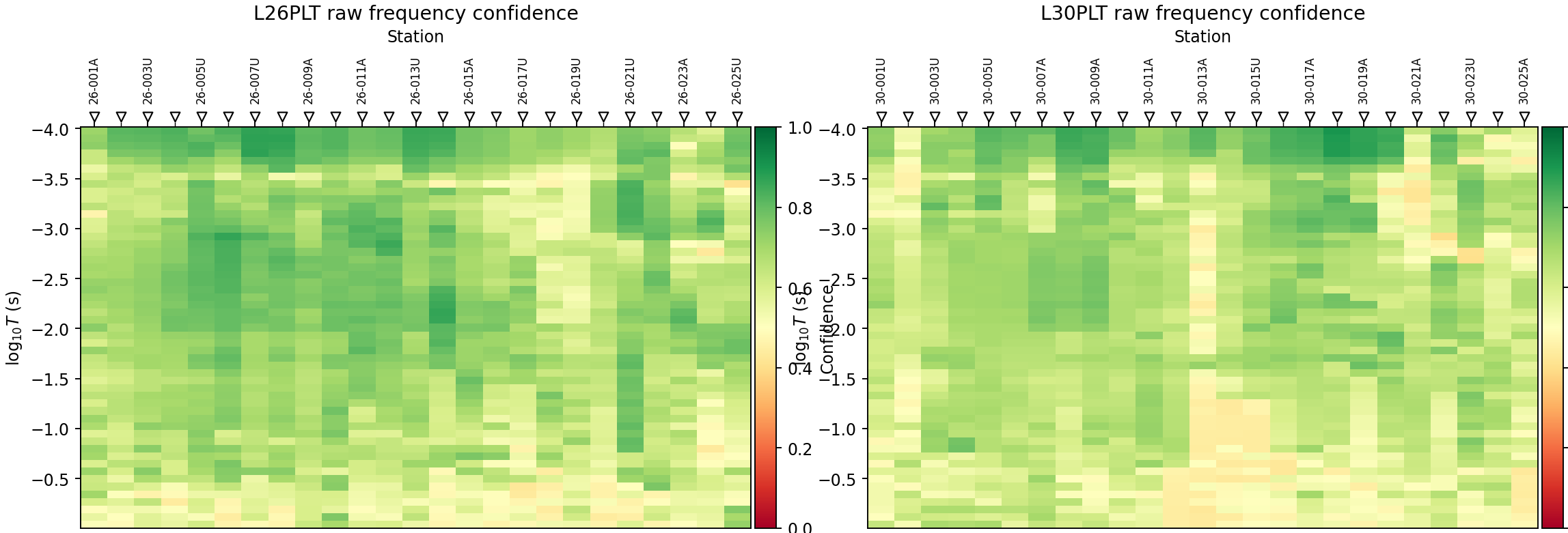
A mean composite confidence around 0.64-0.68 is mediocre, not catastrophic: most station-period rows are usable, but neither line has the uniformly green pseudosection a quiet AMT survey would show. The patchy low-confidence bands sit mostly at short period (high frequency), which is where powerline harmonics live.

18.16.6. Remove Powerline Harmonics

pycsamt.emtools.notch_powerline() targets the 50 Hz mains frequency used at this site (Jiangsu Province, mainland China grid) and its harmonics. The default mode="interp" replaces the affected bins in place by interpolation rather than dropping them, so the row count is unchanged – only the values at the harmonic bins move. The tolerance must reflect the sampled frequency grid: these EDIs contain 50.29 Hz rather than exactly 50.00 Hz, so the former tol_hz=0.06 matched no row and performed no correction. A 0.30 Hz tolerance includes 50.29 Hz without reaching the next logarithmically spaced frequency.

For sampled frequency \(f_i\), mains frequency \(f_m\), harmonic index \(k\), and absolute tolerance \(\epsilon\), the implementation changes a row only when

(2)\[M_i = \mathbf{1}\!\left[ \min_{1\leq k\leq K}|f_i-kf_m|\leq\epsilon \right].\]

With \(\epsilon=0.06\) Hz, equation (2) gives \(M_i=0\) for all 53 rows; with \(\epsilon=0.30\) Hz, it gives \(M_i=1\) at 50.29 Hz and zero elsewhere. This makes the selected correction narrow, explicit, and reproducible rather than visually widening the notch until a difference appears.

>>> from pycsamt.emtools import notch_powerline
>>> import numpy as np
>>> notched26 = notch_powerline(sites26, mains_hz=50.0, n_harm=20, tol_hz=0.30, recursive=False)
>>> notched30 = notch_powerline(sites30, mains_hz=50.0, n_harm=20, tol_hz=0.30, recursive=False)
>>> from pycsamt.emtools._core import _get_z_block
>>> def largest_notch_change(before, after):
...     records = []
...     for raw, corrected in zip(before, after):
...         _, z_raw, freq = _get_z_block(raw)
...         _, z_corrected, _ = _get_z_block(corrected)
...         relative = np.abs(z_corrected[:, 0, 1] - z_raw[:, 0, 1]) / np.maximum(np.abs(z_raw[:, 0, 1]), 1e-30)
...         row = int(np.nanargmax(relative))
...         records.append((float(relative[row]), raw.name, float(freq[row])))
...     change, station, frequency = max(records)
...     return station, round(frequency, 2), round(100.0 * change, 1)
>>> largest_notch_change(sites26, notched26)
('26-001A', 50.29, 68.2)
>>> largest_notch_change(sites30, notched30)
('30-023U', 50.29, 82.1)

Plot that largest single-station change in context – both the local spectrum around 50 Hz and how it compares against every other station on the line – rather than trusting one number in isolation:

import numpy as np
import matplotlib.pyplot as plt
from pycsamt.emtools._core import _get_z_block

fig, axes = plt.subplots(2, 2, figsize=(13.0, 7.2), constrained_layout=True)
for col, (name, before, after) in enumerate(zip(
    ["L26PLT", "L30PLT"], [sites26, sites30], [notched26, notched30]
)):
    records = []
    for ed_before, ed_after in zip(before, after):
        _, zb, fr = _get_z_block(ed_before)
        _, za, _ = _get_z_block(ed_after)
        rel = np.abs(za[:, 0, 1] - zb[:, 0, 1]) / np.maximum(np.abs(zb[:, 0, 1]), 1e-30)
        records.append((float(np.nanmax(rel)), ed_before, ed_after, rel))

    max_rel, ed_before, ed_after, rel = max(records, key=lambda item: item[0])
    _, zb, fr = _get_z_block(ed_before)
    _, za, _ = _get_z_block(ed_after)
    local = (fr >= 20.0) & (fr <= 130.0)
    changed = int(np.nanargmax(rel))

    ax = axes[0, col]
    ax.loglog(fr[local], np.abs(zb[local, 0, 1]), "o-", ms=5, label="raw", color="0.45")
    ax.loglog(fr[local], np.abs(za[local, 0, 1]), "s--", ms=5, label="interpolated", color="crimson")
    ax.axvline(fr[changed], color="#2471a3", linestyle=":", linewidth=1.2)
    ax.set_ylabel("|Zxy|")
    ax.set_title(f"{name} {ed_before.name}: {100 * max_rel:.1f}% at {fr[changed]:.2f} Hz")
    ax.legend(fontsize=8)

    ax = axes[1, col]
    station_change = [100.0 * record[0] for record in records]
    ax.bar(np.arange(len(station_change)), station_change, color="#2471a3")
    ax.set_xlabel("Chainage-ordered station index")
    ax.set_ylabel("max |delta Zxy| / |Zxy| (%)")
    ax.set_title(f"{name}: correction across all stations")
fig.savefig("willy_powerline_notch_before_after.png", dpi=170)

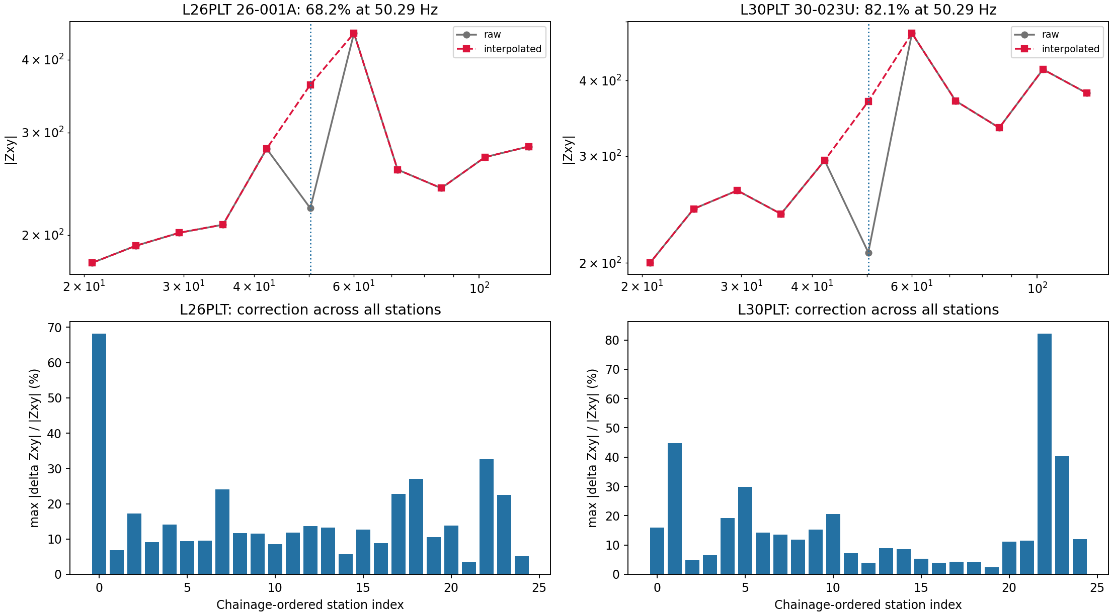
The upper panels deliberately zoom around the 50 Hz fundamental and select the station with the largest change on each line; the vertical marker makes the interpolated 50.29 Hz row visible instead of compressing it into the full 1 Hz–10.4 kHz range. The lower panels show that this is not merely a cosmetic change at two chosen stations: every bar is computed independently from one chainage-ordered station. Large peaks identify stations for which the raw 50.29 Hz impedance departed most strongly from its log-frequency neighbours, while small bars show where interpolation leaves an already smooth local spectrum nearly unchanged.

18.16.7. Dimensionality Dictionary

pycsamt.emtools.learn_dim_dictionary() learns a small set of atoms from phase-tensor features (skew, ellipticity, determinant resistivity, and tipper amplitude where available) by sparse coding, then pycsamt.emtools.encode_dimensionality() labels every station-period row against that learned dictionary rather than a fixed skew/ellipticity threshold.

>>> from pycsamt.emtools import learn_dim_dictionary, encode_dimensionality
>>> model26 = learn_dim_dictionary(notched26, n_atoms=6, lam=0.05, n_iter=40, code_iter=50, recursive=False)
>>> enc26 = encode_dimensionality(notched26, model26, recursive=False, api=True).to_pandas()
>>> enc26["dim_pred"].value_counts().to_dict()
{2: 927, 1: 398}
>>> model30 = learn_dim_dictionary(notched30, n_atoms=6, lam=0.05, n_iter=40, code_iter=50, recursive=False)
>>> enc30 = encode_dimensionality(notched30, model30, recursive=False, api=True).to_pandas()
>>> enc30["dim_pred"].value_counts().to_dict()
{2: 965, 1: 360}

Label 1 (moderate skew, low ellipticity) makes up roughly a quarter to a third of each line (30 percent of L26PLT, 27 percent of L30PLT) and label 2 (the higher-skew/higher-ellipticity atom) the rest; no row on either line lands in the cleanest label 0. That is consistent with the wide but real skew range already seen – most rows still carry enough skew or ellipticity to read as 3-D-flavoured or noisy, but a genuine minority sit in the calmer label 1 rather than every row looking equally disturbed.

import matplotlib.pyplot as plt
from pycsamt.emtools import plot_dim_confidence_grid

fig, axes = plt.subplots(1, 2, figsize=(13.5, 4.8), constrained_layout=True)
for ax, name, sites in zip(axes, ["L26PLT", "L30PLT"], [notched26, notched30]):
    plot_dim_confidence_grid(sites, recursive=False, ax=ax)
    ax.set_title(f"{name} dimensionality confidence")
fig.savefig("willy_dim_confidence_grid.png", dpi=170)

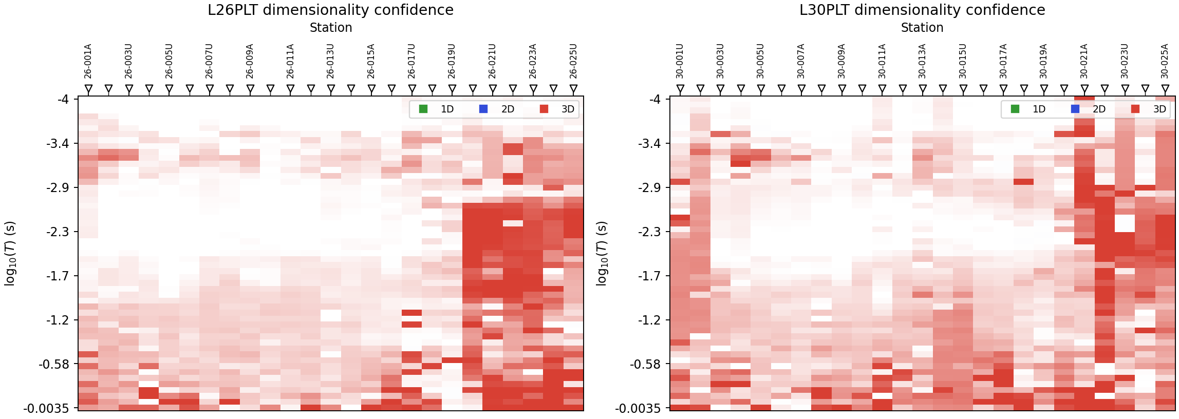
Both lines look broadly similar here, which matters for the next section: neither line has an obvious quiet sub-domain that a simple station filter could isolate. Distortion correction has to be applied line-wide.

18.16.8. Remove Galvanic Distortion

pycsamt.emtools.groom_bailey_table() fits the classic Groom-Bailey decomposition

(3)\[\mathbf{Z}_{\mathrm{obs}}(f) \approx \mathbf{D}\,\mathbf{Z}_{2D}(f),\]

where \(\mathbf{D}\) is a real, frequency-independent distortion matrix and \(\mathbf{Z}_{2D}\) is anti-diagonal at every frequency. The fit reports twist and shear directly; gain is normalized to 1 by construction, because gain and static shift are not separable from the tensor shape alone – resolving the scalar amplitude is exactly what the dedicated static-shift step further below is for.

>>> from pycsamt.emtools import groom_bailey_table, apply_groom_bailey
>>> gb26 = groom_bailey_table(notched26, min_freq=4, robust=True, recursive=False, api=True).to_pandas()
>>> gb_corr26 = apply_groom_bailey(notched26, table=gb26, inplace=False, recursive=False)
>>> ok26 = gb26[gb26["status"] == "ok"]
>>> round(ok26["twist_deg"].median(), 2), round(ok26["shear"].median(), 4)
(2.8, -0.0028)
>>> round(ok26["diagonal_ratio_before"].median(), 3), round(ok26["diagonal_ratio_after"].median(), 3)
(0.345, 0.359)
>>> gb30 = groom_bailey_table(notched30, min_freq=4, robust=True, recursive=False, api=True).to_pandas()
>>> gb_corr30 = apply_groom_bailey(notched30, table=gb30, inplace=False, recursive=False)
>>> ok30 = gb30[gb30["status"] == "ok"]
>>> round(ok30["twist_deg"].median(), 2), round(ok30["shear"].median(), 4)
(8.73, -0.2585)
>>> round(ok30["diagonal_ratio_before"].median(), 3), round(ok30["diagonal_ratio_after"].median(), 3)
(0.487, 0.333)

The line-median twist is mild on both lines, but medians hide the stations that matter. Six stations reach a twist beyond 40 degrees on L26PLT alone (26-020A at 60.3, 26-023A at -49.8, 26-019U at -49.5, 26-025U at 42.2, 26-002A at 25.2, 26-001A at 19.7), and L30PLT has an even larger cluster (30-025A 60.7, 30-013A 55.7, 30-002A 48.8). L30PLT’s larger median diagonal-ratio drop (0.487 to 0.333, versus L26PLT’s 0.345 to 0.359) says the correction is doing more real work there.

from pycsamt.emtools.advanced import plot_distortion_radar

for name, sites, gb in [("L26PLT", notched26, gb26), ("L30PLT", notched30, gb30)]:
    worst = (
        gb.reindex(gb["twist_deg"].abs().sort_values(ascending=False).index)
        .head(6)["station"]
        .tolist()
    )
    fig = plot_distortion_radar(
        sites, stations=worst, max_stations=6, recursive=False,
        title=f"{name}: 6 largest-twist stations",
    )
    fig.savefig(f"willy_{name.lower()}_distortion_radar.png", dpi=170, bbox_inches="tight")

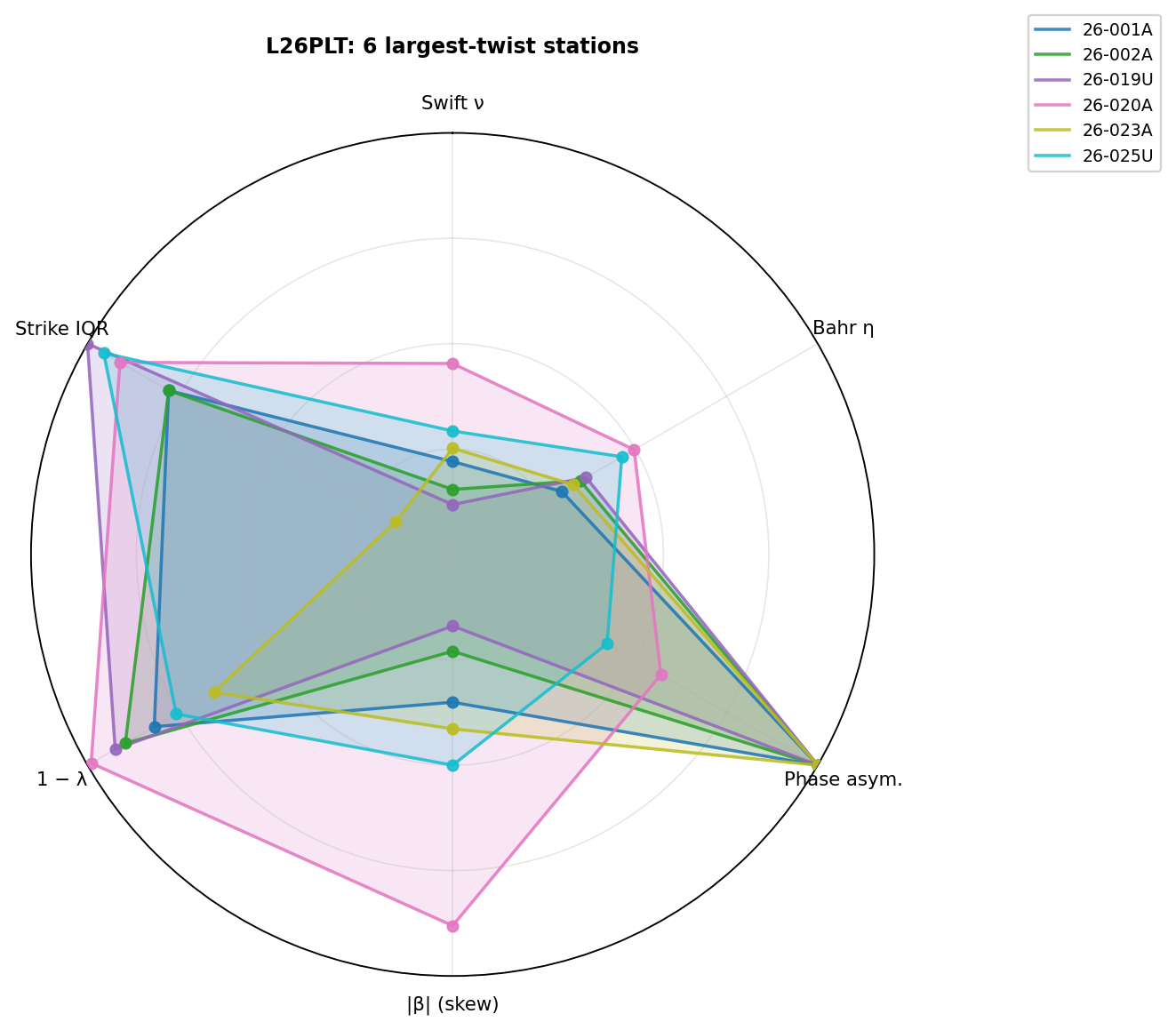
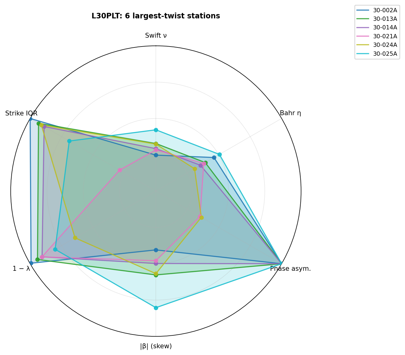
Each polygon is one station’s six-axis distortion fingerprint (Swift skew, Bahr eta, phase asymmetry, PT beta, ellipticity, and dimensionality proxy). Stations that stretch out along several axes at once, not just one, are the ones where a purely scalar static-shift correction would under-describe what is actually happening to the tensor.

18.16.9. Correct Static Shift

pycsamt.emtools.detect_near_surface() separates a frequency-independent scalar shift (the classic static shift model, \(\rho_a'=\rho_a/g\)) from a frequency-dependent near-surface effect that static-shift correction cannot fix. The default f_split=1.0 Hz boundary assumes a broadband MT-style survey reaching well below 1 Hz; WILLY’s audio-band floor sits at 1.008 Hz, so almost nothing would fall below the default split. f_split=50.0 instead splits the band near its geometric centre, and max_skew=None keeps every row – the default 6-degree skew ceiling would reject nearly all of this survey outright, given the skew range already seen.

>>> from pycsamt.emtools import detect_near_surface
>>> ns26 = detect_near_surface(gb_corr26, f_split=50.0, max_skew=None, recursive=False, api=True).to_pandas()
>>> ns26["distortion_type"].value_counts().to_dict()
{'mixed': 17, 'static': 8}
>>> ns30 = detect_near_surface(gb_corr30, f_split=50.0, max_skew=None, recursive=False, api=True).to_pandas()
>>> ns30["distortion_type"].value_counts().to_dict()
{'static': 13, 'mixed': 12}

Neither line has a single clean station by this classification – consistent with everything found so far – but the split between static, near_surface, and mixed matters: it decides how much correction each station gets next.

>>> from pycsamt.emtools import estimate_ss_ama, apply_ss_factors
>>> import numpy as np
>>> factors26 = estimate_ss_ama(gb_corr26, sort_by="name", half_window=3, max_skew=None, recursive=False, api=True).to_pandas()
>>> factors26 = factors26.merge(ns26[["station", "distortion_type"]], on="station", how="left")
>>> factors26["fac_z_reviewed"] = np.where(
...     factors26["distortion_type"].isin(["clean"]), 1.0,
...     factors26["fac_z"].clip(lower=0.3, upper=3.0),
... )
>>> factors26[["station", "fac_z", "distortion_type", "fac_z_reviewed"]].iloc[[0, 15, 19, 20]].round(3)
    station  fac_z distortion_type  fac_z_reviewed
0   26-001A  0.565          static           0.565
15  26-016A  0.840          static           0.840
19  26-020A  0.464           mixed           0.464
20  26-021U  2.107          static           2.107

>>> reviewed26 = factors26[["station", "fac_z_reviewed"]].rename(columns={"fac_z_reviewed": "fac_z"})
>>> ss_corr26 = apply_ss_factors(gb_corr26, reviewed26, key="fac_z", inplace=False, recursive=False)

The clip at [0.3, 3.0] is a review guard, not blanket correction – every station here already qualified as static, mixed, or near_surface, so every factor is applied; a fully clean station would instead be pinned at 1.0 (no change), which is what the np.where branch is for. 26-021U still gets a large 2.11x scaler even after clipping, which is exactly the kind of factor that deserves a note in a production project rather than silent acceptance.

>>> factors30 = estimate_ss_ama(gb_corr30, sort_by="name", half_window=3, max_skew=None, recursive=False, api=True).to_pandas()
>>> factors30 = factors30.merge(ns30[["station", "distortion_type"]], on="station", how="left")
>>> factors30["fac_z_reviewed"] = np.where(
...     factors30["distortion_type"].isin(["clean"]), 1.0,
...     factors30["fac_z"].clip(lower=0.3, upper=3.0),
... )
>>> reviewed30 = factors30[["station", "fac_z_reviewed"]].rename(columns={"fac_z_reviewed": "fac_z"})
>>> ss_corr30 = apply_ss_factors(gb_corr30, reviewed30, key="fac_z", inplace=False, recursive=False)
>>> round(factors30["fac_z_reviewed"].median(), 3)
0.535

With static-shift factors computed and applied for both lines, visualize the resulting log-resistivity shift as a pseudosection instead of reading it off a table:

import matplotlib.pyplot as plt
from pycsamt.emtools import plot_ss_delta_psection

fig, axes = plt.subplots(1, 2, figsize=(13.5, 5.0), constrained_layout=True)
plot_ss_delta_psection(gb_corr26, ss_corr26, ax=axes[0])
axes[0].set_title("L26PLT static-shift delta log10(rho)")
plot_ss_delta_psection(gb_corr30, ss_corr30, ax=axes[1])
axes[1].set_title("L30PLT static-shift delta log10(rho)")
fig.savefig("willy_static_shift_delta.png", dpi=170)

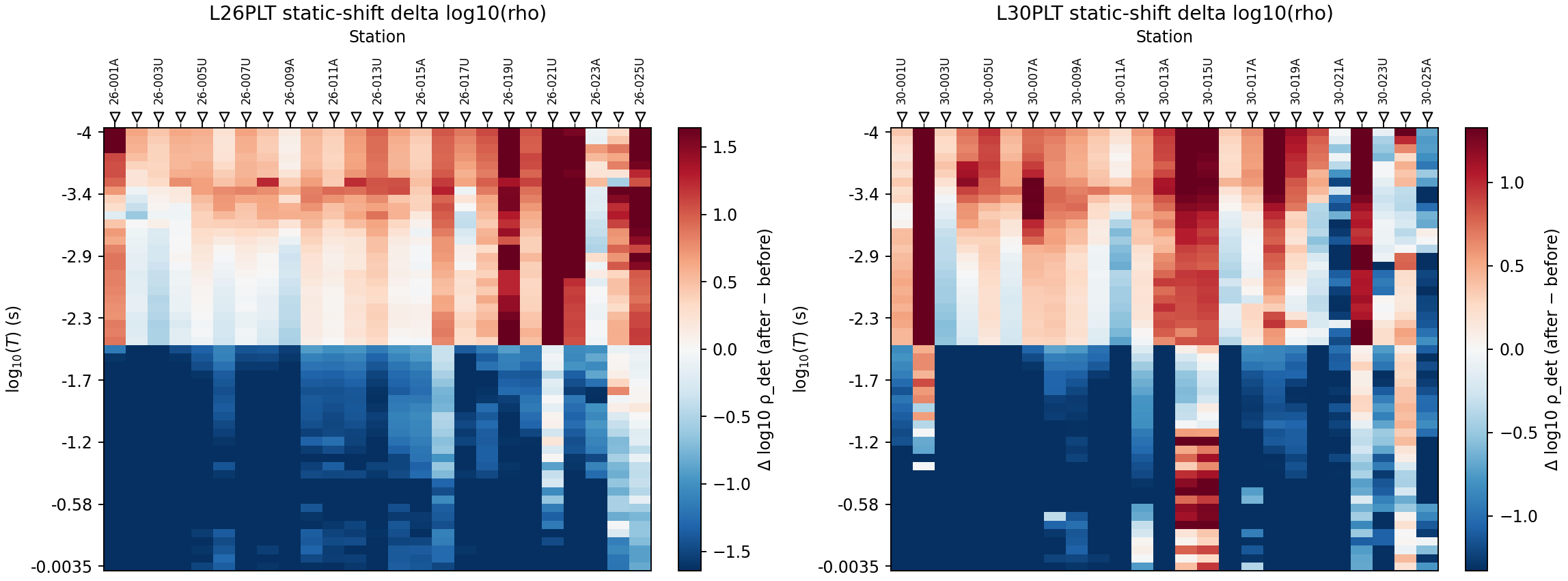
The delta is constant with period at any one station – the visual signature of a genuinely scalar correction – and its sign and size vary station to station in the same patchy way the QC table already showed. That patchiness, not a smooth trend, is what a static-shift-dominated line looks like.

18.16.10. EMAP Spatial Filter

Static shift and Groom-Bailey both work station by station. What is left after both is spatially incoherent noise that only shows up when neighbouring stations are compared directly – pycsamt.emtools.apply_emap_filter() implements two profile-wide options, AMA and FLMA, worth comparing rather than picking blindly.

>>> from pycsamt.emtools import apply_emap_filter
>>> ama26 = apply_emap_filter(ss_corr26, method="ama", window_m=1500.0, spacing_m=200.0, comp="det", inplace=False, recursive=False)
>>> flma26 = apply_emap_filter(ss_corr26, method="flma", window=5, component="all", inplace=False, recursive=False)

>>> def rho_xy_all(ss):
...     from pycsamt.emtools._core import _iter_items, _get_z_block
...     out = []
...     for ed in _iter_items(ss):
...         _, z, fr = _get_z_block(ed)
...         if z is None:
...             continue
...         rho = 0.2 * np.abs(z[:, 0, 1]) ** 2 / np.maximum(fr, 1e-30)
...         out.append(rho[np.isfinite(rho) & (rho > 0)])
...     return np.concatenate(out)
...
>>> r0, ra, rf = rho_xy_all(ss_corr26), rho_xy_all(ama26), rho_xy_all(flma26)
>>> round(np.std(np.log10(r0)), 4), round(np.std(np.log10(ra)), 4), round(np.std(np.log10(rf)), 4)
(1.0364, 0.9598, 0.8924)

Both filters reduce the log-resistivity spread; FLMA reduces it further on L26PLT (0.892 versus AMA’s 0.960, down from an unfiltered 1.036). The same comparison on L30PLT gives 0.954 (FLMA) versus 0.967 (AMA) against an unfiltered 1.066 – FLMA wins on both lines, so it is the production choice below.

>>> flma30 = apply_emap_filter(ss_corr30, method="flma", window=5, component="all", inplace=False, recursive=False)

With FLMA now applied to both lines, plot the before/after/delta pseudosection that the comparison above was based on:

from pycsamt.emtools import plot_emap_filter_psection

for name, before, after in [("L26PLT", ss_corr26, flma26), ("L30PLT", ss_corr30, flma30)]:
    fig = plot_emap_filter_psection(before, after, method="flma", component="xy")
    fig.savefig(f"willy_{name.lower()}_emap_flma_psection.png", dpi=170, bbox_inches="tight")

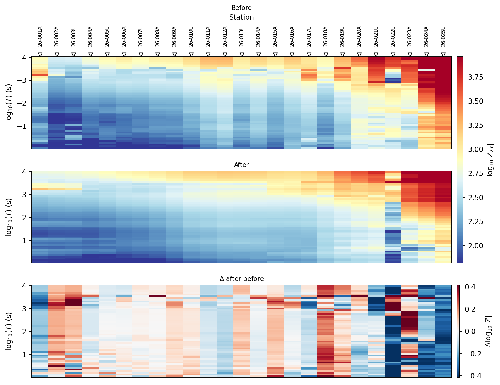
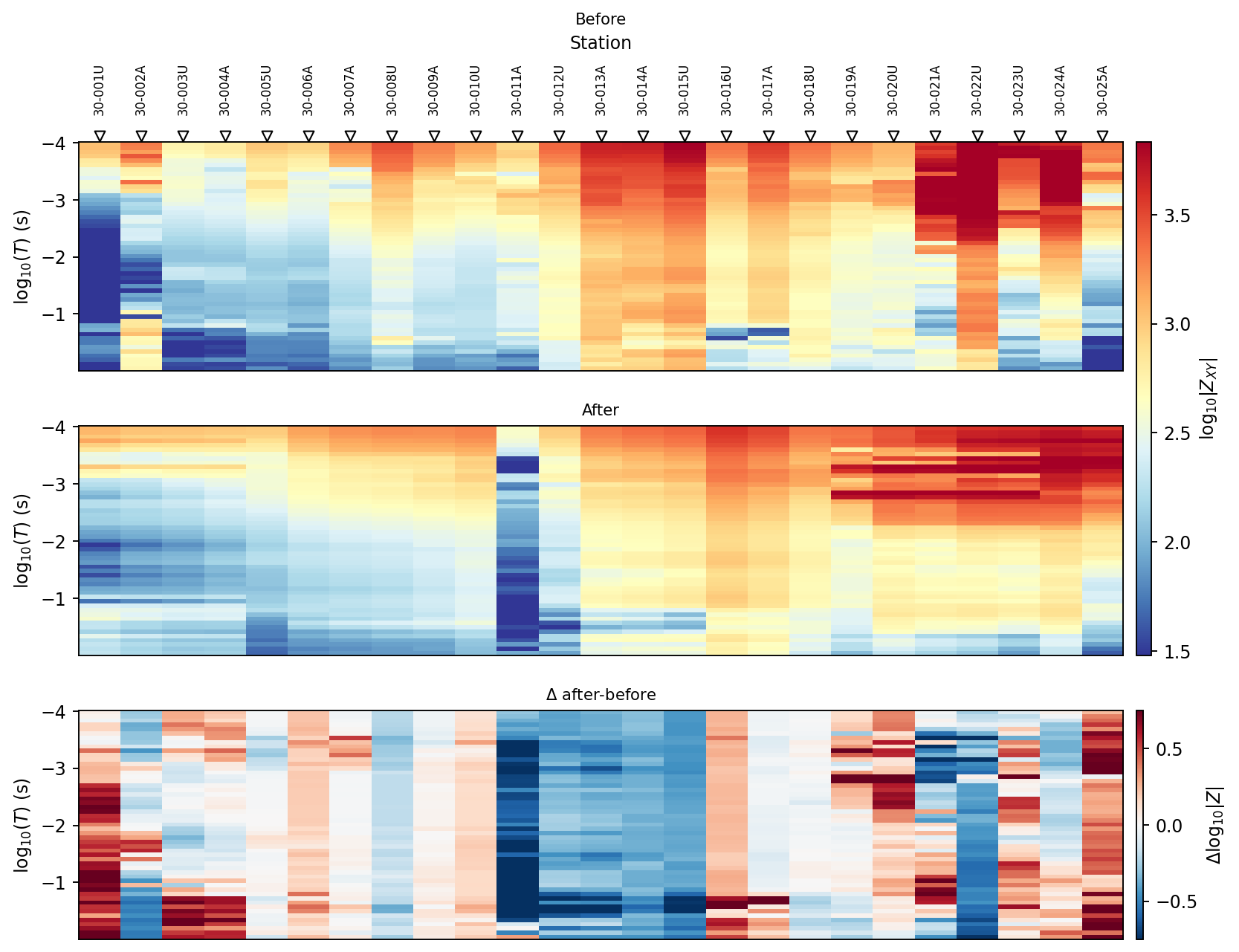
The delta panel is where the filter’s actual footprint lives: it is small and scattered, not a broad smooth wash across the whole line, which is the desired behaviour for a filter meant to suppress incoherent noise without also erasing genuine lateral structure.

18.16.11. Drop Weak Frequencies

The QC pass at the start flagged individual station-period rows as weak; pycsamt.emtools.drop_low_confidence_frequencies() removes them now, after every tensor-level correction, so the confidence scores reflect the corrected data rather than the raw one.

>>> from pycsamt.emtools import drop_low_confidence_frequencies
>>> dropped26 = drop_low_confidence_frequencies(flma26, method="composite", threshold=0.5, also="both", inplace=False, recursive=False)
>>> dropped30 = drop_low_confidence_frequencies(flma30, method="composite", threshold=0.5, also="both", inplace=False, recursive=False)

Visualize exactly which station-period rows each line lost to this threshold, rather than trusting the aggregate percentage alone:

import matplotlib.pyplot as plt
from pycsamt.emtools import plot_frequency_edit_summary

fig, axes = plt.subplots(1, 2, figsize=(13.5, 4.6), constrained_layout=True)
plot_frequency_edit_summary(flma26, dropped26, ax=axes[0])
axes[0].set_title("L26PLT bad-frequency drop (threshold=0.5)")
plot_frequency_edit_summary(flma30, dropped30, ax=axes[1])
axes[1].set_title("L30PLT bad-frequency drop (threshold=0.5)")
fig.savefig("willy_bad_frequency_drop_summary.png", dpi=170)

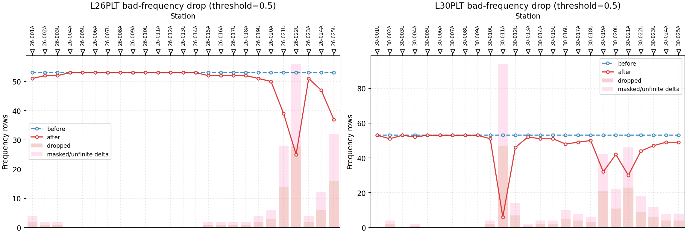
L26PLT loses 79 of 1325 station-frequency rows (about 6.0 percent); L30PLT loses 154 (about 11.6 percent). One L30PLT station, 30-011A, drops from 53 usable frequencies to only 5 – a station worth flagging for manual review or exclusion in a production project, not silently carried forward at face value.

The corrected, sanitized survey is exported to disk here, ready to be reloaded independently by every remaining section:

>>> from pycsamt.agents.edi_export import EDIExportAgent
>>> r26 = EDIExportAgent(overwrite=True).execute({"sites": dropped26, "output_dir": "runs/L26PLT_corrected"})
>>> r26.status, r26.data["n_written"]
('success', 25)
>>> r30 = EDIExportAgent(overwrite=True).execute({"sites": dropped30, "output_dir": "runs/L30PLT_corrected"})
>>> r30.status, r30.data["n_written"]
('success', 25)

18.16.12. Skew And Dimensionality

Reload the corrected EDIs and check whether the correction chain actually changed the skew and dimensionality picture, rather than assuming it.

>>> from pycsamt.api import read_edis
>>> corr26 = Sites(read_edis("runs/L26PLT_corrected", recursive=False, strict=False, progress=False).collection).ordered("chainage")
>>> corr30 = Sites(read_edis("runs/L30PLT_corrected", recursive=False, strict=False, progress=False).collection).ordered("chainage")
>>> from pycsamt.emtools import build_phase_tensor_table
>>> pt26 = build_phase_tensor_table(corr26, recursive=False)
>>> len(pt26), round(pt26["beta"].abs().median(), 2), round(pt26["beta"].abs().quantile(0.9), 2)
(1246, 13.05, 45.44)
>>> pt30 = build_phase_tensor_table(corr30, recursive=False)
>>> len(pt30), round(pt30["beta"].abs().median(), 2), round(pt30["beta"].abs().quantile(0.9), 2)
(1171, 15.15, 53.25)

The correction chain removes powerline spikes, galvanic distortion, static shift, incoherent noise, and weak rows – it does not, and should not, manufacture a low-skew line out of genuinely 3-D or noisy data. A median skew around 13-15 degrees after correction is a real improvement over the uncorrected, per-station picture in the Baseline Quality Check above (which ranged as high as 61 degrees): most of the corrected data now sits close to the classical few-degree “clean 2-D” range. The 90th percentile still reaching 45-53 degrees is the honest remainder – correction removes identifiable distortion and noise, it does not manufacture 2-D structure where the earth is genuinely 3-D, and roughly a tenth of the corrected data still reads that way.

import matplotlib.pyplot as plt
from pycsamt.emtools import plot_phase_tensor_skewmap, plot_dimensionality_psection

fig, axes = plt.subplots(2, 2, figsize=(13.5, 8.6), constrained_layout=True)
for col, (name, sites) in enumerate([("L26PLT", corr26), ("L30PLT", corr30)]):
    plot_phase_tensor_skewmap(sites, recursive=False, ax=axes[0, col])
    axes[0, col].set_title(f"{name} phase-tensor skew")
    plot_dimensionality_psection(sites, recursive=False, ax=axes[1, col])
    axes[1, col].set_title(f"{name} dimensionality")
fig.savefig("willy_skew_dimensionality_grid.png", dpi=170)

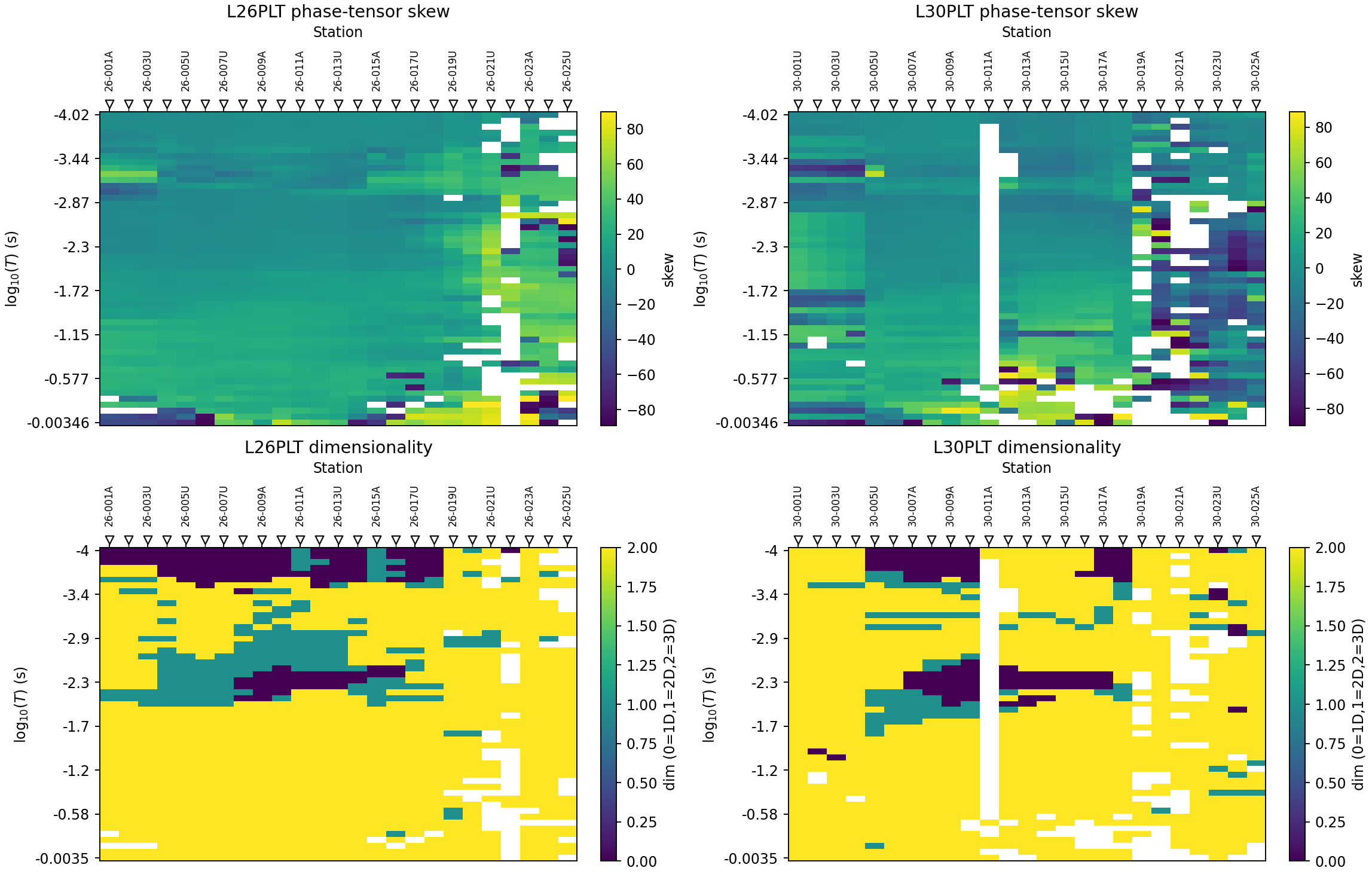
Dimensionality now shows real period-dependent structure rather than a uniform wash: both lines carry a genuine mix of 1-D (dark) and 2-D (teal) labels at short period, concentrated roughly between \(\log_{10}(T)=-4\) and \(-2.3\), before the classification settles into predominantly 3-D (yellow) at longer periods on most stations. Shallower structure reading closer to 1-D/2-D and deeper structure reading more 3-D is exactly the pattern expected approaching a genuinely 3-D porphyry alteration system at depth, rather than a uniform artefact of one leftover processing issue at every period.

18.16.13. Estimate Strike

pycsamt.emtools.estimate_strike_consensus() blends an impedance-tensor rotation sweep with a phase-tensor azimuth estimate into one angle per station; combine the per-station angles into a circular mean.

>>> from pycsamt.emtools import estimate_strike_consensus
>>> consensus26 = estimate_strike_consensus(corr26, recursive=False)
>>> ang26 = consensus26["ang"].dropna().to_numpy()
>>> doubled = np.deg2rad(2.0 * ang26)
>>> dominant26 = 0.5 * np.rad2deg(np.arctan2(np.sin(doubled).mean(), np.cos(doubled).mean()))
>>> round(dominant26, 2)
-36.42
>>> consensus30 = estimate_strike_consensus(corr30, recursive=False)
>>> ang30 = consensus30["ang"].dropna().to_numpy()
>>> doubled = np.deg2rad(2.0 * ang30)
>>> dominant30 = 0.5 * np.rad2deg(np.arctan2(np.sin(doubled).mean(), np.cos(doubled).mean()))
>>> round(dominant30, 2)
-45.84

The circular spread behind each of these means is close to 50 degrees on both lines – broad, not a tight single-domain result. That is worth carrying forward explicitly rather than hiding behind a clean-looking mean angle.

from pycsamt.emtools import plot_strike_analysis

for name, sites in [("L26PLT", corr26), ("L30PLT", corr30)]:
    fig = plot_strike_analysis(
        sites, recursive=False,
        suptitle=f"{name} strike / phase-tensor analysis",
    )
    fig.savefig(f"willy_{name.lower()}_strike_analysis.png", dpi=170, bbox_inches="tight")

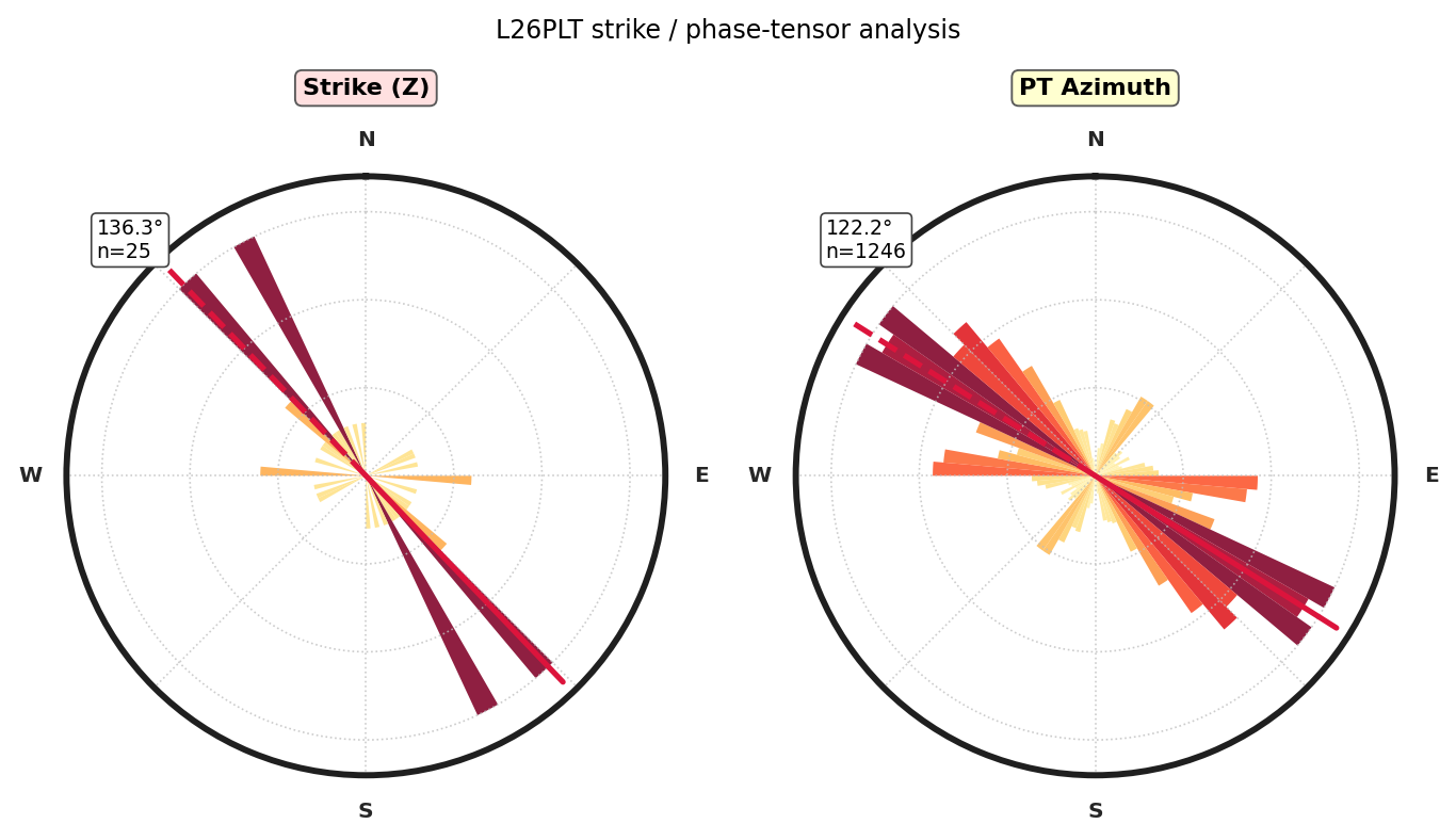
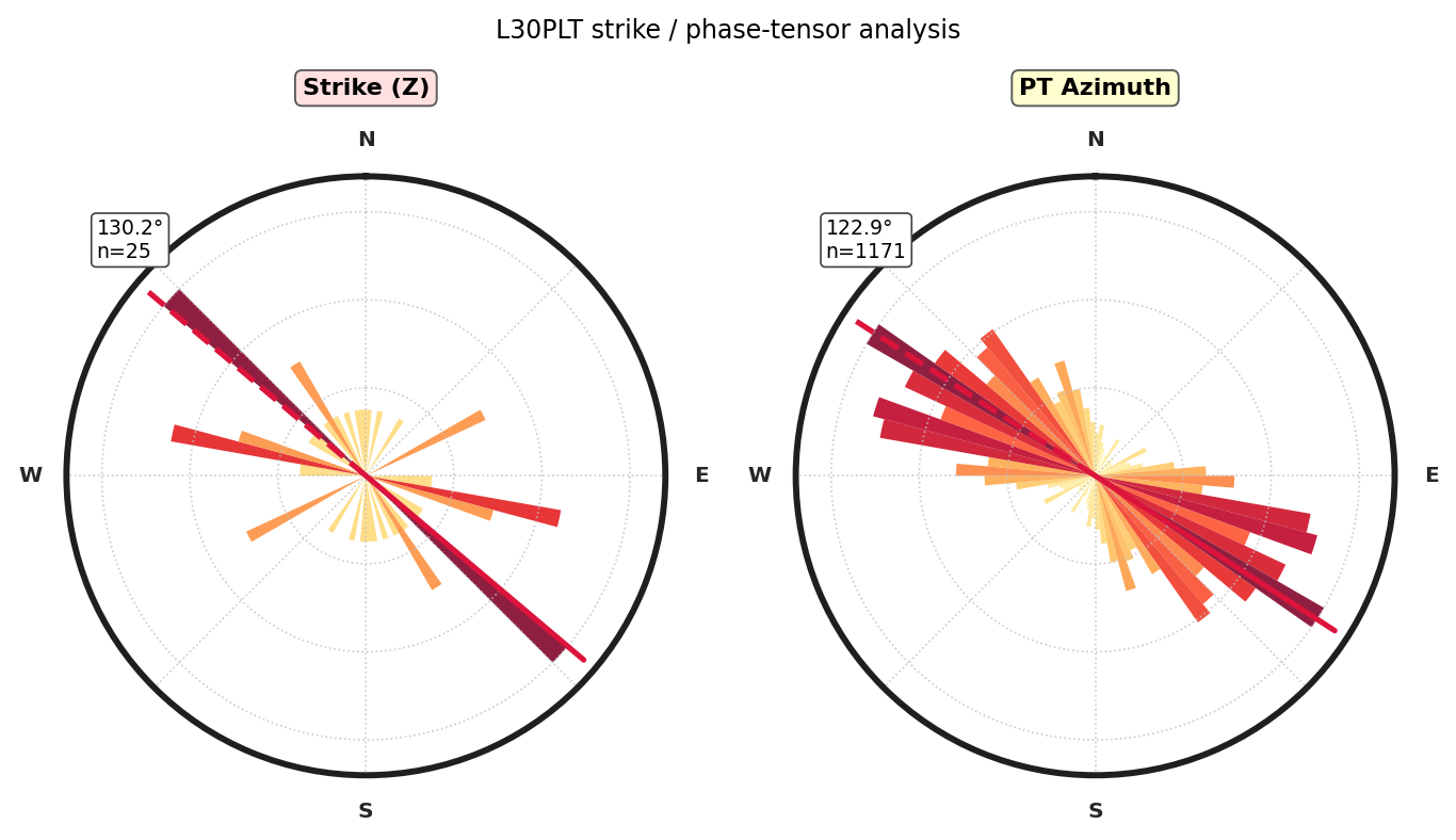
WILLY_DATA carries no vertical-field channel, so plot_strike_analysis() detects that and renders only the two panels it can actually support here – Strike (Z) and PT Azimuth – rather than a third, permanently empty tipper panel. The impedance-sweep and phase-tensor roses agree only loosely with each other on both lines, which matches the broad circular spread already measured and argues against treating either line’s rotation as a precision result.

18.16.14. Rotate To Strike

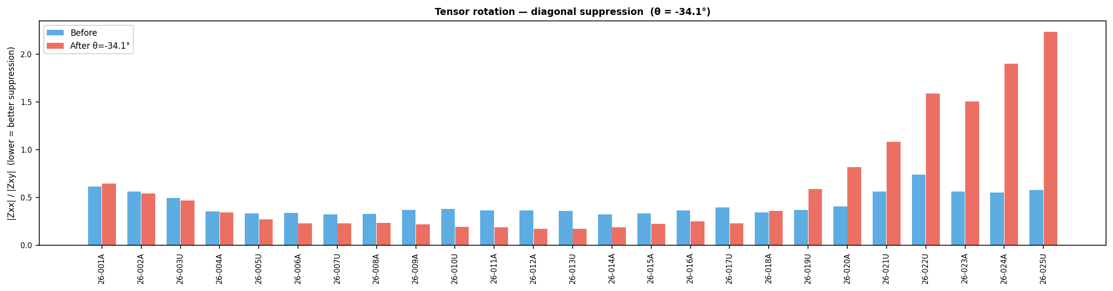
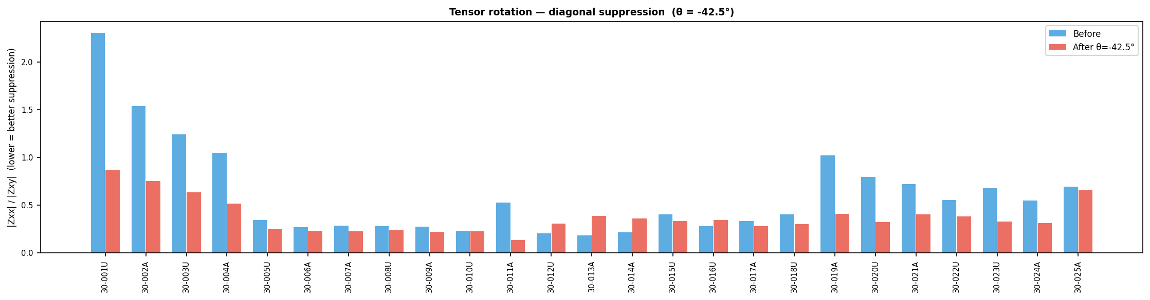
pycsamt.agents.tensor_rotation.TensorRotationAgent rotates impedance to the estimated strike and writes rotated EDI files, and reports a diagonal-suppression check: whether rotating actually reduced \(|Z_{xx}|/|Z_{xy}|\), the signature of successful 2-D alignment.

>>> from pycsamt.agents.tensor_rotation import TensorRotationAgent
>>> agent26 = TensorRotationAgent(strike_deg=-36.42)
>>> rot26 = agent26.execute({"sites": corr26, "output_dir": "runs/L26PLT_rotated", "overwrite": True})
>>> rot26.status, rot26.data["n_written"], round(rot26.data["z_diag_reduction"], 4)
('success', 25, -0.1864)
>>> agent30 = TensorRotationAgent(strike_deg=-45.84)
>>> rot30 = agent30.execute({"sites": corr30, "output_dir": "runs/L30PLT_rotated", "overwrite": True})
>>> rot30.status, rot30.data["n_written"], round(rot30.data["z_diag_reduction"], 4)
('success', 25, 0.2749)

This is the honest outcome of a broad, noisy strike estimate: rotation helps L30PLT (diagonal suppression improves by 0.275) but does not help L26PLT (it gets 0.186 worse, consistently across several period bands and consensus methods tried while preparing this tutorial). Rotating L26PLT anyway keeps the two lines on a comparable classical-inversion footing, but its 2-D/TE-TM split should be trusted less than L30PLT’s; the rotation-free AI 3-D inversion further below is the more appropriate cross-check specifically for L26PLT.

18.16.15. Prepare Occam2D Inputs

With rotated EDIs on disk, pycsamt.models.occam2d.InputBuilder builds a native 2-D input set exactly as in Prepare an Occam2D Inversion, one line at a time.

>>> from pycsamt.api import read_edis
>>> from pycsamt.models.occam2d import OccamConfig, InputBuilder
>>> cfg = OccamConfig(
...     modes=["TE", "TM"], freq_min=1.0, freq_max=10400.0,
...     error_floor_rho=0.05, error_floor_phase=0.5,
...     n_layers=30, n_airlayers=4, cell_size_horizontal=60.0,
...     cell_size_vertical_top=15.0, depth_scale=1.15,
...     target_misfit=1.0, max_iterations=80, initial_rho=100.0,
... )
>>> rot26_sites = Sites(read_edis("runs/L26PLT_rotated", recursive=False, strict=False, progress=False).collection).ordered("chainage")
>>> builder26 = InputBuilder(rot26_sites, workdir="runs/L26PLT_occam2d", config=cfg, verbose=0)
>>> _ = builder26.build(title="L26PLT pyCSAMT porphyry Occam2D preparation")
>>> print(builder26.summary())
InputBuilder summary
  workdir   : runs\L26PLT_occam2d
  sites     : 25
  freqs     : 53
  data pts  : 4984
  mesh      : 62 x 34 cells
  params    : 780
  modes     : ['TE', 'TM']

>>> rot30_sites = Sites(read_edis("runs/L30PLT_rotated", recursive=False, strict=False, progress=False).collection).ordered("chainage")
>>> builder30 = InputBuilder(rot30_sites, workdir="runs/L30PLT_occam2d", config=cfg, verbose=0)
>>> _ = builder30.build(title="L30PLT pyCSAMT porphyry Occam2D preparation")
>>> builder30.data.n_data
4684

Compare how the QC-driven frequency drop shows up in each line’s own Occam2D data-row count before moving on to the mesh those rows share:

import numpy as np
import matplotlib.pyplot as plt

fig, axes = plt.subplots(1, 2, figsize=(13.5, 4.6), constrained_layout=True)
for ax, name, b in zip(axes, ["L26PLT", "L30PLT"], [builder26, builder30]):
    db = b.data.data_blocks
    site_idx = db[:, 1].astype(int)
    comp_codes = db[:, 2].astype(int)
    for code, label in {1: "RhoTE", 2: "PhsTE", 5: "RhoTM", 6: "PhsTM"}.items():
        m = comp_codes == code
        counts = np.bincount(site_idx[m], minlength=len(b.data.sites))
        ax.plot(np.arange(len(counts)), counts, label=label, marker=".", ms=3)
    ax.set_xlabel("Station index")
    ax.set_ylabel("Data rows")
    ax.set_title(f"{name} Occam2D data rows by station")
    ax.legend(fontsize=7)
fig.savefig("willy_occam2d_data_rows.png", dpi=170)

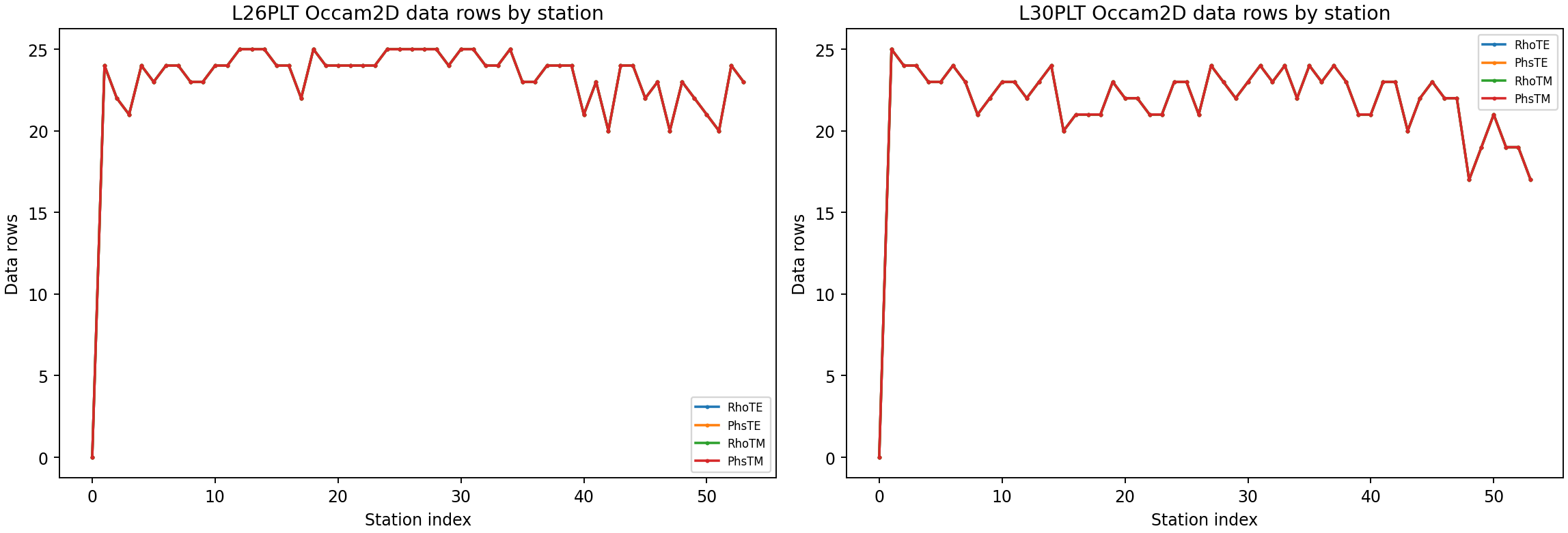
L26PLT carries more data points than L30PLT (4984 versus 4684) purely from the earlier frequency-drop step – L30PLT lost more rows at the QC stage, and Occam2D simply reflects that in its row count.

Both lines share the same mesh design regardless of that row-count difference; plot its cell skeleton to confirm the padding grows smoothly away from the station footprint before treating it as ready for either solver:

fig, axes = plt.subplots(1, 2, figsize=(13.5, 5.0), constrained_layout=True)
for ax, name, b in zip(axes, ["L26PLT", "L30PLT"], [builder26, builder30]):
    mesh = b.mesh
    for xv in mesh.x_nodes:
        ax.axvline(xv, color="0.75", lw=0.4)
    for zv in mesh.z_nodes:
        ax.axhline(zv, color="0.75", lw=0.4)
    ax.set_ylim(mesh.z_nodes[-1], 0)
    ax.set_xlim(mesh.x_nodes[0], mesh.x_nodes[-1])
    ax.set_xlabel("Horizontal (m)")
    ax.set_ylabel("Depth (m)")
    ax.set_title(f"{name} Occam2D mesh ({mesh.n_xcells} x {mesh.n_zcells})")
fig.savefig("willy_occam2d_mesh_skeleton.png", dpi=170)

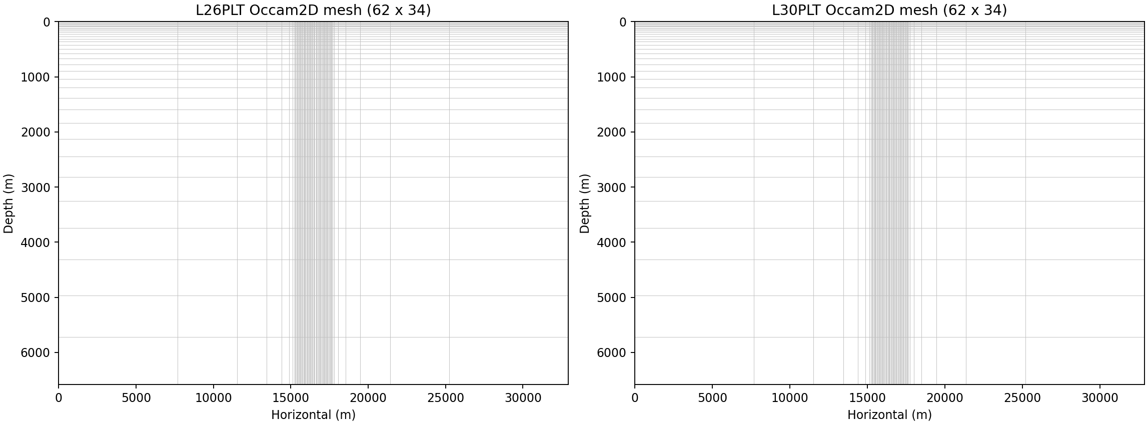
Both lines share the same 62 x 34 cell mesh and 780 parameters, since they use the same OccamConfig. As in Prepare an Occam2D Inversion, this tutorial stops at file preparation and validation; build or locate the occam2d binary first (Occam2D), then run it against runs/L26PLT_occam2d and runs/L30PLT_occam2d separately, and reload each with pycsamt.models.occam2d.InversionResult when a completed run is available.

18.16.16. Prepare ModEM 3-D Inputs

For 3-D, keep the corrected data unrotated – ModEM works directly with a 3-D impedance tensor and does not need TE/TM separation – and combine both lines into a single 3-D survey with pycsamt.models.modem.builder.InputBuilder.

>>> from pycsamt.models.modem import ModEmConfig
>>> from pycsamt.models.modem.builder import InputBuilder as ModEmBuilder
>>> combined = corr26.to_edis() + corr30.to_edis()
>>> len(combined)
50
>>> cfg3d = ModEmConfig(mode="3d", initial_rho=100.0, freq_min=1.0, freq_max=10400.0)
>>> builder3d = ModEmBuilder(config=cfg3d)
>>> files = builder3d.build(combined, workdir="runs/willy_modem_3d")
>>> sorted(files)
['control', 'covariance', 'data', 'model']
>>> builder3d.model.shape
(35, 45, 59)
>>> len(builder3d.data.site_names), len(builder3d.data.periods)
(50, 53)

Inspect how far that starting mesh grows away from the station footprint in each of the three directions before treating it as ready to solve:

import numpy as np
import matplotlib.pyplot as plt

model = builder3d.model
fig, axes = plt.subplots(1, 3, figsize=(13.0, 3.6), constrained_layout=True)
labels = ["x (north-south, m)", "y (east-west, m)", "z (depth, m)"]
widths = [np.diff(model.x_nodes), np.diff(model.y_nodes), np.diff(model.z_nodes)]
for ax, w, lab in zip(axes, widths, labels):
    ax.plot(w, marker=".", ms=3)
    ax.set_title(lab)
    ax.set_xlabel("cell index")
    ax.set_ylabel("width (m)")
fig.suptitle(
    f"ModEM 3-D starting mesh: {model.shape[0]} x {model.shape[1]} x "
    f"{model.shape[2]} cells, {len(builder3d.data.site_names)} stations"
)
fig.savefig("willy_modem3d_mesh_widths.png", dpi=170)

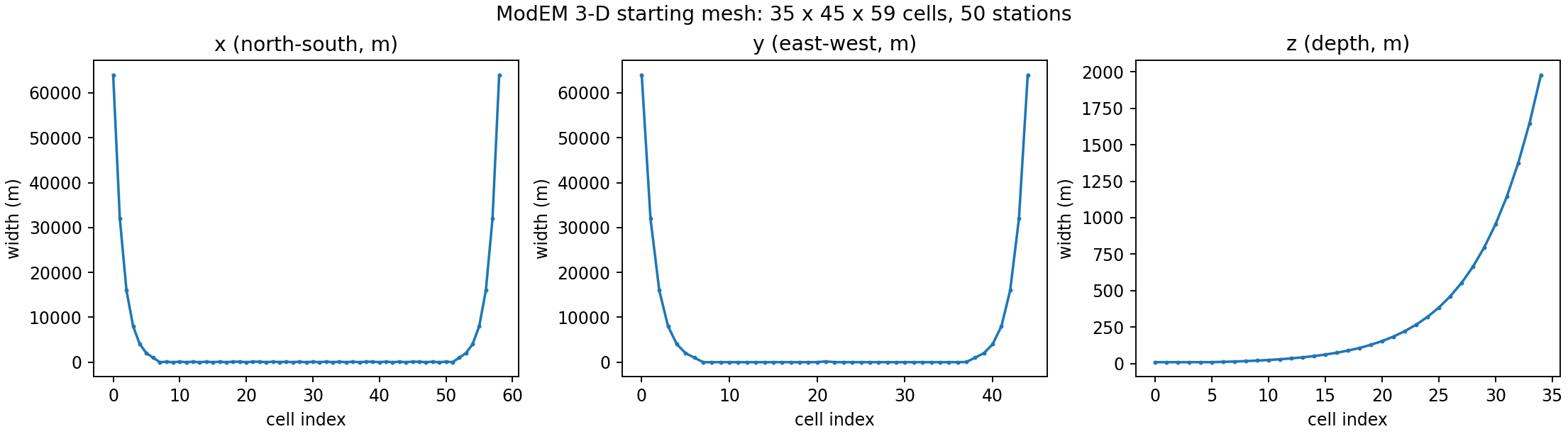
Cell widths grow geometrically away from the station footprint in all three directions, which is the expected padding behaviour for a 3-D inversion mesh – fine cells where the data actually constrain the model, coarse cells further out to satisfy the boundary conditions cheaply.

data.dat, m0.ws, covariance.cov, and control.inv are now in runs/willy_modem_3d. As with the Occam2D lines above, this tutorial stops at file preparation; the actual solve runs outside Python, against a locally compiled Mod3DMT (ModEM covers building it, including the MPI and Intel-build variants). pycsamt.models.modem.ModEmRunner builds that command from the same cfg3d used above, so the launch stays tied to the configuration that generated the files rather than retyped by hand:

>>> from pycsamt.models.modem import ModEmRunner
>>> runner = ModEmRunner("runs/willy_modem_3d", config=cfg3d)
>>> command = runner.command(
...     "m0.ws", "data.dat", "control.inv", covariance="covariance.cov",
... )
>>> print(command)
Mod3DMT -I NLCG m0.ws data.dat control.inv covariance.cov

Set cfg3d.use_mpi = True and cfg3d.n_procs beforehand to get an mpirun -np N ... form instead. Run that command externally, then reload the finished run with pycsamt.models.modem.InversionResult and plot it with pycsamt.models.modem.PlotModel3D. ModEM covers the full ModEM workflow – configuration, native files, the runner, and diagnostics – against a bundled, already-converged sample run.

18.16.17. Maxwell-Trained 2-D AI Inversion of Both Lines

The corrected EDI folders are now the input boundary for AI inversion. Keep the two profiles separate: a 2-D forward operator assumes invariance normal to one profile, and concatenating L26 and L30 would create a fictitious connection between their end stations. Each line therefore receives its own geological hypothesis, topographic surface, padded Maxwell mesh, training dataset, model, and validation record.

The geology is a seeded prior, not an interpretation of these data. For line \(l\), its cell model is

(4)\[\log_{10}\rho_l(x,z)= \log_{10}\bar{\rho}_{k_l(x,z)}+ \sigma_{k_l(x,z)}g_l(x,z),\]

where \(k_l\) is the stratigraphic unit, \(g_l\) is a correlated Gaussian field, and an optional ellipsoid represents a conductive target hypothesis. Seeds 2601 and 3001 make the two realizations repeatable without forcing them to be identical. In a real study, train over an ensemble of plausible interfaces, correlations, bodies, and resistivities rather than selecting the realization that most resembles the expected target.

The following short excerpt shows the public objects. The complete two-line implementation—including loading, model construction, inversion, validation, and plotting—is exposed as a copyable accordion below.

>>> from pycsamt.ai.geology import (
...     ElectricalLayer, EllipsoidalLens, GaussianCorrelation,
...     GeologyGrid, generate_layered_geology, insert_lenses,
...     topography_from_sites,
... )
>>> from pycsamt.forward.maxwell import MeshDesign, build_solver_mesh
>>> grid26 = GeologyGrid.regular_2d(
...     nx=30, nz=24, dx_m=100, dz_m=75, x_origin_m=-250,
... )
>>> topography26 = topography_from_sites(
...     corr26, grid26, profile_origin_m=-250,
... )
>>> grid26.shape, round(topography26.relief_m, 1)
((24, 30), 162.0)

The terrain object is supplied to pycsamt.forward.maxwell.build_solver_mesh(), which classifies earth and air before solving. Topography is therefore part of the numerical domain; it is not painted onto a flat result afterward. Padding keeps artificial boundaries away from the receiver footprint, while the quality record checks cell ratios and resolution against skin depth.

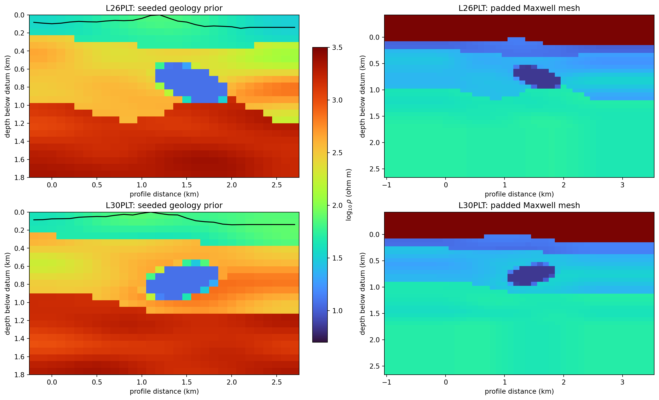
The left column contains two different, explicitly hypothetical geology realizations. The right column shows how each becomes a solver model: resistive numerical air occupies the cells above terrain and geometrically growing padding surrounds the 2.4 km receiver footprint. Both resulting meshes have 33 x 38 = 1254 cells. Similar geometry does not imply the same geology; it only reflects the shared discretization policy.

18.16.17.1. Run genuine 2-D training physics

Set physics="mt2d" explicitly. Omitting it selects the legacy mt1d mode, which tiles independent 1-D responses and cannot validate lateral Maxwell physics. Matching n_stations_per_profile to all 25 field stations also prevents silent truncation.

>>> import numpy as np
>>> from pycsamt.agents import Inv2DAgent
>>> frequencies_hz = np.geomspace(1.0, 1000.0, 8)
>>> agent26 = Inv2DAgent(
...     physics="mt2d", n_depth=24, depth_max=1800,
...     n_freqs=8, freqs=frequencies_hz,
...     n_train_profiles=100, n_stations_per_profile=25,
...     station_spacing_m=101.5, epochs=100,
...     correlation_length_x_m=(350, 1000),
...     correlation_length_z_m=(90, 300),
...     lambda_x=.02, lambda_z=.01, lambda_tv=.005,
... )
>>> result26 = agent26.execute({
...     "sites": corr26,
...     "topography": True,
...     "output_dir": "runs/L26PLT_ai2d_maxwell",
... })
>>> result26.status, result26.data["physics"]
('success', 'mt2d')
>>> result26.data["pred_section"].shape
(24, 25)

Instantiate a second agent with the L30 median station spacing and write to a different output directory. Do not reuse a trained L26 network as though it were an independent L30 inversion: that would couple experiments without recording the dependency.

The training objective combines supervised model recovery with declared spatial penalties,

(5)\[\mathcal{J}(\theta)= \frac{1}{N}\sum_{i=1}^{N} \left\|f_\theta(\mathbf d_i)-\mathbf m_i\right\|_2^2 +\lambda_x\|D_x\hat{\mathbf m}_i\|_2^2 +\lambda_z\|D_z\hat{\mathbf m}_i\|_2^2 +\lambda_{TV}\operatorname{TV}(\hat{\mathbf m}_i),\]

where every \(\mathbf d_i\) is generated by the verified 2-D Maxwell adapter from known model \(\mathbf m_i\). Regularization discourages unsupported oscillation; it does not prove that a recovered feature is real.

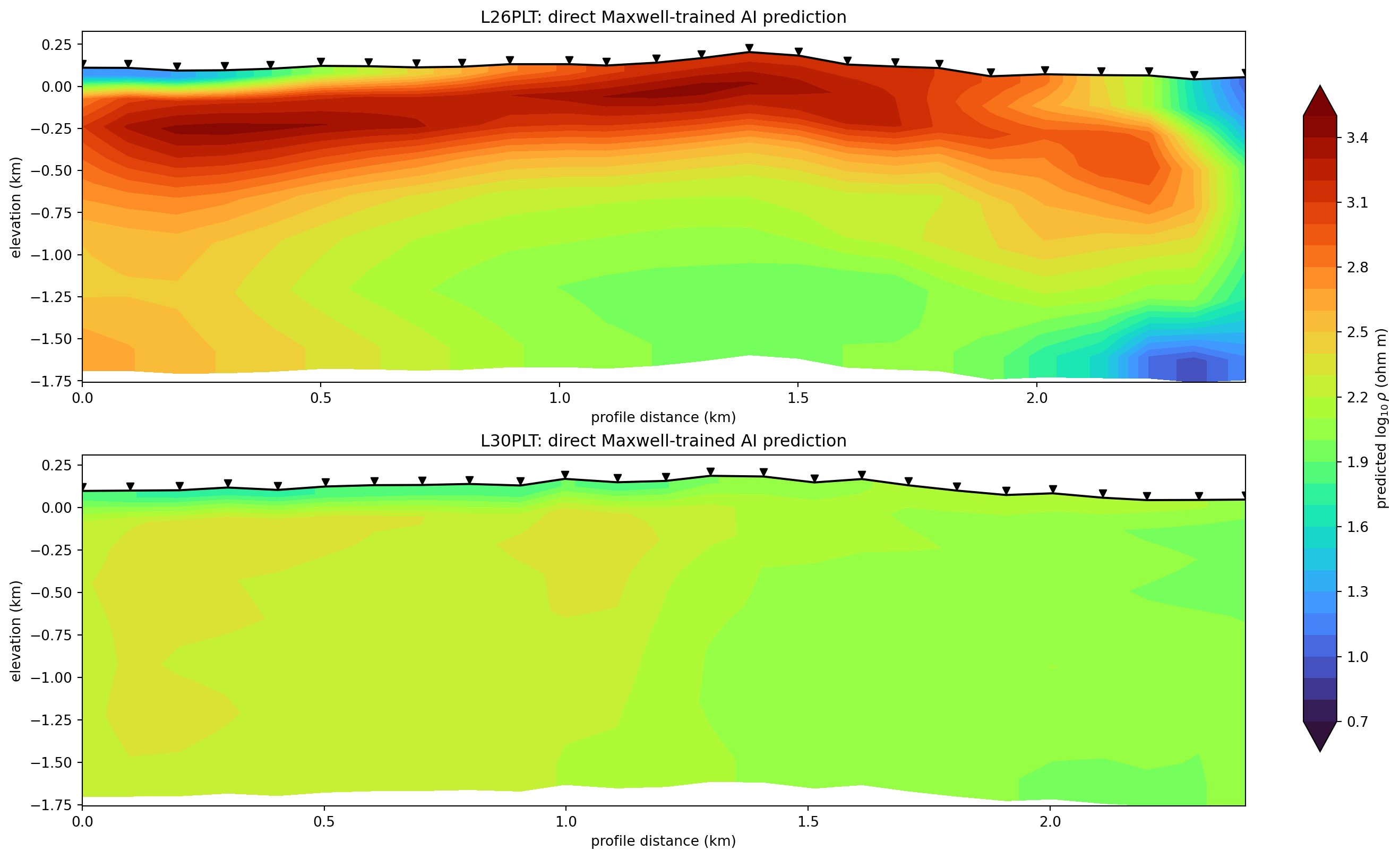
These are the direct pred_section arrays on the agent-returned 1.8 km depth axis—no pseudosection blending, trend injection, smoothing, or invented depth conversion is used. At this larger training scale, L26 develops a coherent, near-continuous resistive cap (\(\log_{10}\rho\) up to about 3.5) spanning most of the profile in the top 0.3 km, transitioning to a mid-range background (\(\log_{10}\rho\simeq2.0\)) at depth, plus a localized low-resistivity patch (\(\log_{10}\rho\) below 1) near the deep right edge of the section (2.1--2.4 km chainage). L30 stays comparatively featureless, hovering close to the mean prediction near \(\log_{10}\rho\simeq2.0\)–2.3 with only mild local texture. The contrast demonstrates what the model actually learned, but—as the gate below still confirms—it is not sufficient evidence to label either pattern as alteration or mineralization.

18.16.17.2. Gate the result before interpretation

Global RMS tests response consistency, whereas held-out recovery tests whether the network reconstructs known geological models outside its fitting subset. They answer different questions and both must pass a threshold chosen before viewing the field model.

>>> round(result26.data["rms_global"], 3)
1.31
>>> recovery26 = result26.data["mt2d_recovery"]
>>> round(recovery26["rmse"], 3), recovery26["n_samples"]
(0.482, 10)

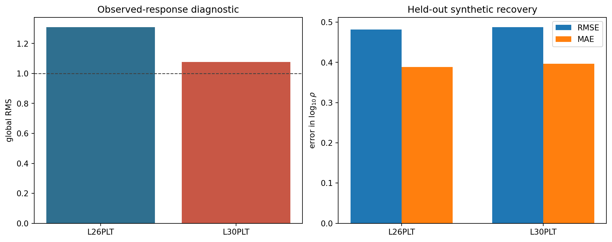
L26 and L30 reach response RMS 1.310 and 1.077, respectively, while recovery RMSE is 0.482 and 0.488 log10 ohm m, evaluated over 10 held-out samples per line rather than one. The larger held-out set makes these error estimates noticeably more trustworthy than the earlier ten- realization run, but recovery \(R^2\) is still barely positive (0.063 and 0.045)—far below the 0.60 acceptance threshold—and 10 samples remains short of the 20-sample floor set below. L26’s added structure makes the figure more useful pedagogically, whereas L30’s near-uniform prediction exposes the remaining limitation. Both still fail the structural-recovery gate and therefore do not support a drilling interpretation.

Raising n_train_profiles from 10 to 100 and epochs from 30 to 100 improved recovery \(R^2\) from effectively zero to a small positive value and grew the held-out set from 1 to 10 samples, but it did not clear the gate—confirming that more of the same eight-frequency, correlated-field training recipe is not enough on its own. The next correct step is to strengthen the training dataset and rerun both lines, publishing replacement sections only after structural recovery passes. For this survey, a meaningful rerun should use 200--500+ Maxwell geology realizations, 16--32 retained frequencies, and an upper limit of 30--100 epochs with validation-based early stopping. It should also cover broader layered, lens, fault/contact, and correlated-field priors; repeat multiple seeds; evaluate recovery by depth and target; and verify that the synthetic response distribution overlaps the L26/L30 observations.

18.16.17.3. Tune this configuration for a real deployment

Everything on this page, including the 100-realization rerun above, is deliberately sized for documentation-build time, not for a defensible field interpretation. If you are adapting this workflow for your own survey, treat the table below as a starting checklist of what to widen and why, then read the detailed reasoning that follows it before committing CPU time.

What to change before trusting a result

Parameter	This page (demo)	Widen toward	Why
n_train_profiles	100	200--500+	Populates train/val/test splits and grows the held-out set past the 20-sample gate floor; this is the dominant cost driver (see below).
epochs (ceiling)	100	30--100	Already near the useful range; early stopping (patience = max(5, epochs // 5)) restores the best checkpoint on its own, so raising this further rarely helps once patience is already tuned.
frequencies	8 (1–1000 Hz)	16--32	Match the field survey’s own QC-surviving band; four isolated decades under-samples the response compared to the field data.
n_depth / depth_max	24 / 1800 m	32 / 2200 m	More vertical degrees of freedom, kept within the survey’s real investigation depth—do not extend past what the frequency band resolves.
correlation lengths / resistivity priors	narrow, single family	wider ranges; add layered/lens/fault families explicitly	The convenience agent only samples one correlated-field family; broader priors and explicit geology objects (below) prevent the network from overfitting to an unrealistically narrow training distribution.
mesh_safety_factor / max_mesh_cells	6.0 / 200,000	8.0 / 300,000	Only matters if the quality diagnostics show resolution against skin depth is marginal; verify before spending the extra mesh cells.
root seed	one (17)	repeat [17, 29, 43, 71, 101]	A feature that moves between seeds is unstable, not real.
promotion thresholds	fixed below	fix before viewing the field result	rmse <= 0.25, r2 >= 0.60, n_samples >= 20 is an example policy; choose your own in advance and do not adjust it after looking.

Budget the compute before choosing these numbers. Fitting the checkpointed loss-curve lengths against the elapsed times measured on this page shows that generating each Maxwell realization costs roughly 32 CPU-seconds on this 25-station, 8-frequency, 1254-cell mesh, while training costs well under 0.1 CPU-seconds per realization-epoch once early stopping is active. Concretely, that means raising n_train_profiles is what makes a rerun expensive, not raising epochs—a 500-realization run at similar mesh/frequency complexity costs on the order of 500 * 32 s ≈ 4.4 CPU-hours per line just to generate the training data, before any of the [17, 29, 43, 71, 101] seed repeats multiply that further. The practical levers are: parallelize realization generation across cores (each Maxwell solve is independent), cache a generated dataset and reuse it across epoch/regularization sweeps instead of regenerating it every run, and only pay for a denser frequency grid or larger mesh once the quality diagnostics show they are actually the resolution bottleneck.

The following project-scale agent configuration makes the changes that the current convenience API exposes directly:

>>> project_frequencies = np.geomspace(1.0, 10_000.0, 24)
>>> production_agent = Inv2DAgent(
...     physics="mt2d",
...     n_depth=32,
...     depth_max=2200.0,
...     n_freqs=len(project_frequencies),
...     freqs=project_frequencies,
...     n_train_profiles=256,
...     n_stations_per_profile=25,
...     station_spacing_m=101.5,
...     epochs=80,
...     correlation_length_x_m=(250.0, 1600.0),
...     correlation_length_z_m=(60.0, 450.0),
...     log_resistivity_mean=2.1,
...     log_resistivity_std=0.75,
...     lambda_x=0.01,
...     lambda_z=0.005,
...     lambda_tv=0.002,
...     mesh_safety_factor=8.0,
...     max_mesh_cells=300_000,
... )

n_train_profiles=256 replaces ten examples by enough realizations to populate training, validation, and test partitions. It does not guarantee coverage, so inspect the split counts and response distributions. The 24 frequencies sample four decades instead of four isolated values; for another survey, derive this vector from the frequencies that survived QC rather than copying the bounds blindly. Increasing n_depth to 32 gives the network more vertical degrees of freedom, while depth_max=2200 keeps them within the survey’s intended investigation range.

epochs=80 is a ceiling, not a requirement to train for all 80 epochs. pycsamt.agents.Inv2DAgent automatically uses validation patience max(5, epochs // 5)—16 epochs here—and restores the best state. The wider correlation-length and log-resistivity distributions expose the network to compact and regional structures and a substantially broader resistivity range. Because the standardized Gaussian field is not hard bounded, inspect empirical quantiles and impose scientifically justified limits in a custom dataset when extreme resistivities would be implausible. The smaller regularization weights still suppress isolated pixels but are less likely to erase a recovered body; choose them from validation sweeps, not from the field image.

The convenience Inv2DAgent currently generates correlated-field geology. It does not yet turn the separately constructed LayeredGeology and EllipsoidalLens objects above into its training ensemble. To include layered, lens, fault/contact, and multiple-body families, generate those realizations explicitly with pycsamt.ai.geology, solve every one through pycsamt.forward.maxwell, preserve their models/responses in the dataset contract, and fit pycsamt.ai.inversion.EMInverter2D directly. Merely raising n_train_profiles repeats the configured correlated-field family; it does not broaden geological support.

Repeat the complete experiment with independent root seeds, for example [17, 29, 43, 71, 101]. A feature is unstable when its position or amplitude changes materially between accepted seeds. Do not average failed runs into an apparently smooth final section.

Before promotion, require all predeclared checks—not just low field RMS:

>>> recovery = result26.data["mt2d_recovery"]
>>> response_pass = result26.data["rms_global"] <= 1.2
>>> recovery_pass = recovery["rmse"] <= 0.25 and recovery["r2"] >= 0.60
>>> enough_test_models = recovery["n_samples"] >= 20
>>> promote = response_pass and recovery_pass and enough_test_models
>>> promote
False

The numerical thresholds are an example acceptance policy and must be fixed before inspecting the field result. Add depth-resolved RMSE, conductor-boundary overlap, anomaly-centroid error, predicted-versus-observed response panels, and out-of-distribution tests. Better agreement between training and observations means overlap in frequency/component availability, apparent-resistivity and phase ranges, noise/error distributions, station spacing, topographic relief, and expected geological scales—not merely similar global means.

The configuration above is no longer a quick integration test at this scale. On the documentation machine, training both lines at 100 realizations with an epochs=100 ceiling took 3,554.7 s (L26PLT) and 3,473.4 s (L30PLT)—7,028 s combined, or about 117 minutes. Validation-based early stopping (patience max(5, epochs // 5) = 20) did trigger in both runs, well short of the 100-epoch ceiling: L26PLT stopped after 38 epochs (best validation loss 0.968), L30PLT after 28 (0.970). Wall-clock time is nevertheless dominated by generating the 100 Maxwell realizations themselves, not by training on them—fitting the checkpointed loss-curve lengths against elapsed time gives roughly 32 CPU-seconds per realization generated versus well under 0.1 CPU-seconds per realization-epoch trained. The earlier 10-realization, 30-epoch run took only 813.8 s combined for both lines, consistent with that same per-realization cost. Practically, this means raising n_train_profiles is what makes a rerun expensive here, not raising epochs. The aspirational 256-realizations-per-line production configuration below, with three times the frequencies and a larger mesh, is a substantially bigger job again and was not run for this page. Record the dataset configuration, split manifest, seeds, mesh diagnostics, loss curves, held-out metrics, and observed-response residuals for each line.

</>View and copy the complete L26/L30 Maxwell-AI workflowClick to inspect and copy the complete code

"""Run and plot the two-line Maxwell-AI workflow used by the porphyry tutorial."""

from __future__ import annotations

import argparse
import json
import random
import sys
import time
from pathlib import Path

import matplotlib

matplotlib.use("Agg")
import matplotlib.pyplot as plt
import numpy as np

ROOT = Path(__file__).resolve().parents[2]
sys.path.insert(0, str(ROOT))

from pycsamt.agents import Inv2DAgent  # noqa: E402
from pycsamt.ai.geology import (  # noqa: E402
    ElectricalLayer,
    EllipsoidalLens,
    GaussianCorrelation,
    GeologyGrid,
    generate_layered_geology,
    insert_lenses,
    topography_from_sites,
)
from pycsamt.emtools import ensure_sites  # noqa: E402
from pycsamt.forward.maxwell import MeshDesign, build_solver_mesh  # noqa: E402
from pycsamt.topo import extract_chainage, extract_elevation  # noqa: E402

IMAGE_DIR = ROOT / "docs/source/images/tutorials/map_porphyry_mineralization_from_noisy_amt"
RUN_DIR = ROOT / "runs"
FREQUENCIES_HZ = np.geomspace(1.0, 1000.0, 8)
PRODUCTION_FREQUENCIES_HZ = np.geomspace(1.0, 10_000.0, 24)


def save(fig: plt.Figure, name: str) -> None:
    IMAGE_DIR.mkdir(parents=True, exist_ok=True)
    fig.savefig(IMAGE_DIR / name, dpi=190, bbox_inches="tight")
    plt.close(fig)


def load_lines():
    lines = {}
    for name in ("L26PLT", "L30PLT"):
        corrected = RUN_DIR / f"{name}_corrected"
        if not corrected.exists():
            raise FileNotFoundError(
                f"{corrected} is missing; run the tutorial's correction/export steps first."
            )
        lines[name] = ensure_sites(corrected, recursive=False, verbose=0).ordered()
    return lines


def build_line_problem(name, sites, *, seed, lens_x_m):
    chain_m = extract_chainage(sites) * 1000.0
    dx = 100.0
    x_origin = -250.0
    nx = int(np.ceil((chain_m[-1] + 500.0) / dx))
    grid = GeologyGrid.regular_2d(
        nx=nx, nz=24, dx_m=dx, dz_m=75.0, x_origin_m=x_origin
    )
    correlation = GaussianCorrelation(700.0, 160.0)
    layers = [
        ElectricalLayer("weathered cover", 45.0, 0.10, correlation),
        ElectricalLayer("altered intrusive", 350.0, 0.16, correlation),
        ElectricalLayer("fresh intrusive", 1600.0, 0.10, correlation),
    ]
    base = generate_layered_geology(
        grid,
        layers,
        [320.0, 1050.0],
        seed=seed,
        interface_relief_std_m=[45.0, 100.0],
        interface_correlation=correlation,
        minimum_thickness_m=120.0,
    )
    target = EllipsoidalLens(
        f"{name} conductive target",
        center_x_m=lens_x_m,
        center_z_m=760.0,
        radius_x_m=480.0,
        radius_z_m=210.0,
        resistivity_ohm_m=12.0,
        dip_deg=18.0 if name == "L26PLT" else -12.0,
        transition_fraction=0.20,
    )
    geology = insert_lenses(base, [target])
    topography = topography_from_sites(
        sites, grid, profile_origin_m=x_origin, interpolation_method="linear"
    )
    solver_model = build_solver_mesh(
        grid,
        resistivity_ohm_m=geology.resistivity_ohm_m,
        frequencies_hz=FREQUENCIES_HZ,
        topography=topography,
        design=MeshDesign(
            horizontal_padding_cells=4,
            bottom_padding_cells=5,
            air_layers=4,
            padding_expansion=1.3,
        ),
    )
    return {
        "name": name,
        "sites": sites,
        "chain_m": chain_m,
        "grid": grid,
        "geology": geology,
        "topography": topography,
        "solver_model": solver_model,
    }


def plot_priors_and_meshes(problems) -> None:
    fig, axes = plt.subplots(2, 2, figsize=(13.6, 8.2), constrained_layout=True)
    for row, problem in enumerate(problems):
        grid = problem["grid"]
        topo = problem["topography"]
        geology = problem["geology"]
        mesh_model = problem["solver_model"]
        im = axes[row, 0].pcolormesh(
            grid.x_m / 1000.0,
            grid.z_m / 1000.0,
            np.log10(geology.resistivity_ohm_m),
            cmap="turbo", vmin=0.7, vmax=3.5, shading="auto",
        )
        axes[row, 0].plot(
            grid.x_m / 1000.0, topo.surface_depth_m / 1000.0, "k", lw=1.4
        )
        axes[row, 0].invert_yaxis()
        axes[row, 0].set(
            title=f"{problem['name']}: seeded geology prior",
            xlabel="profile distance (km)", ylabel="depth below datum (km)",
        )
        x = mesh_model.mesh.cell_centres_m["x"] / 1000.0
        z = mesh_model.mesh.cell_centres_m["z"] / 1000.0
        axes[row, 1].pcolormesh(
            x, z, np.log10(1.0 / mesh_model.conductivity_s_m),
            cmap="turbo", vmin=0.7, vmax=8.0, shading="auto",
        )
        axes[row, 1].invert_yaxis()
        axes[row, 1].set(
            title=f"{problem['name']}: padded Maxwell mesh",
            xlabel="profile distance (km)", ylabel="depth below datum (km)",
        )
    fig.colorbar(im, ax=axes[:, 0], shrink=.82, label=r"$\log_{10}\rho$ (ohm m)")
    save(fig, "willy_ai2d_geology_maxwell_both_lines.png")


def run_inversions(
    problems,
    *,
    production: bool = False,
    n_train_profiles: int | None = None,
    epochs: int | None = None,
):
    np.random.seed(17)
    random.seed(17)
    try:
        import torch

        torch.manual_seed(17)
    except ImportError:
        pass
    results = []
    for problem in problems:
        chain = problem["chain_m"]
        spacing = float(np.median(np.diff(chain)))
        frequencies = (
            PRODUCTION_FREQUENCIES_HZ if production else FREQUENCIES_HZ
        )
        profiles = int(
            n_train_profiles
            if n_train_profiles is not None
            else (256 if production else 10)
        )
        epoch_budget = int(
            epochs if epochs is not None else (80 if production else 30)
        )
        line_output = RUN_DIR / (
            f"{problem['name']}_ai2d_maxwell_production"
            if production
            else f"{problem['name']}_ai2d_maxwell"
        )
        line_output.mkdir(parents=True, exist_ok=True)
        started = time.time()
        agent = Inv2DAgent(
            physics="mt2d",
            n_depth=32 if production else 24,
            n_freqs=len(frequencies),
            freqs=frequencies,
            depth_max=2200.0 if production else 1800.0,
            n_train_profiles=profiles,
            n_stations_per_profile=len(problem["sites"]),
            station_spacing_m=spacing,
            epochs=epoch_budget,
            correlation_length_x_m=(250.0, 1600.0) if production else (350.0, 1000.0),
            correlation_length_z_m=(60.0, 450.0) if production else (90.0, 300.0),
            log_resistivity_mean=2.1,
            log_resistivity_std=0.75 if production else 0.5,
            lambda_x=0.01 if production else 0.02,
            lambda_z=0.005 if production else 0.01,
            lambda_tv=0.002 if production else 0.005,
            mesh_safety_factor=8.0 if production else 6.0,
            max_mesh_cells=300_000 if production else 200_000,
        )
        result = agent.execute(
            {
                "sites": problem["sites"],
                "output_dir": str(line_output),
                "topography": True,
            }
        )
        if result.status != "success":
            raise RuntimeError(f"{problem['name']}: {result.summary}")
        checkpoint = line_output / "em_inverter_2d_maxwell.npz"
        result.data["inverter"].save(checkpoint)
        np.savez_compressed(
            line_output / "field_prediction.npz",
            pred_section=np.asarray(result.data["pred_section"]),
            depths_km=np.asarray(result.data["depths_km"]),
            frequency_grid_hz=np.asarray(result.data["frequency_grid_hz"]),
            station_names=np.asarray(result.data["station_names"]),
            chainage_km=np.asarray(problem["chain_m"]) / 1000.0,
            elevation_m=extract_elevation(problem["sites"]),
        )
        recovery = result.data.get("mt2d_recovery") or {}
        manifest = {
            "line": problem["name"],
            "status": result.status,
            "summary": result.summary,
            "production": production,
            "seed": 17,
            "n_train_profiles": profiles,
            "epochs_requested": epoch_budget,
            "n_depth": 32 if production else 24,
            "depth_max_m": 2200.0 if production else 1800.0,
            "frequencies_hz": frequencies.tolist(),
            "rms_global": float(result.data["rms_global"]),
            "mt2d_recovery": recovery,
            "elapsed_seconds": time.time() - started,
            "checkpoint": checkpoint.name,
        }
        (line_output / "run_manifest.json").write_text(
            json.dumps(manifest, indent=2, default=float), encoding="utf-8"
        )
        print(json.dumps(manifest, default=float), flush=True)
        results.append(result)
    return results


def plot_inversions(problems, results) -> None:
    fig, axes = plt.subplots(2, 1, figsize=(13.8, 8.4), constrained_layout=True)
    images = []
    for ax, problem, result in zip(axes, problems, results):
        section = np.asarray(result.data["pred_section"], dtype=float)
        depth_km = np.asarray(result.data["depths_km"], dtype=float)
        chain_km = problem["chain_m"] / 1000.0
        elevation_km = extract_elevation(problem["sites"]) / 1000.0
        reference = float(np.max(elevation_km))
        z = reference - depth_km[:, None] + (elevation_km - reference)[None, :]
        x = np.broadcast_to(chain_km[None, :], section.shape)
        image = ax.contourf(
            x, z, section, levels=np.linspace(.7, 3.5, 29),
            cmap="turbo", vmin=.7, vmax=3.5, extend="both",
        )
        images.append(image)
        ax.plot(chain_km, elevation_km, "k", lw=1.5)
        ax.scatter(chain_km, elevation_km + .025, marker="v", c="k", s=24)
        ax.set(
            title=f"{problem['name']}: direct Maxwell-trained AI prediction",
            xlabel="profile distance (km)", ylabel="elevation (km)",
        )
    fig.colorbar(images[0], ax=axes, shrink=.86, label=r"predicted $\log_{10}\rho$ (ohm m)")
    save(fig, "willy_ai2d_maxwell_predictions_both_lines.png")


def plot_validation(problems, results) -> None:
    names = [p["name"] for p in problems]
    rms = [float(r.data["rms_global"]) for r in results]
    recovery = [r.data.get("mt2d_recovery") or {} for r in results]
    rmse = [float(r.get("rmse", np.nan)) for r in recovery]
    mae = [float(r.get("mae", np.nan)) for r in recovery]
    fig, axes = plt.subplots(1, 2, figsize=(10.8, 4.2), constrained_layout=True)
    axes[0].bar(names, rms, color=["#2f6f8f", "#c85745"])
    axes[0].axhline(1, color="0.25", ls="--", lw=1)
    axes[0].set(title="Observed-response diagnostic", ylabel="global RMS")
    x = np.arange(2)
    axes[1].bar(x - .18, rmse, .36, label="RMSE")
    axes[1].bar(x + .18, mae, .36, label="MAE")
    axes[1].set_xticks(x, names)
    axes[1].set(title="Held-out synthetic recovery", ylabel=r"error in $\log_{10}\rho$")
    axes[1].legend()
    save(fig, "willy_ai2d_maxwell_validation_both_lines.png")


def main(argv: list[str] | None = None) -> int:
    parser = argparse.ArgumentParser()
    parser.add_argument("--production", action="store_true")
    parser.add_argument("--n-train-profiles", type=int)
    parser.add_argument("--epochs", type=int)
    args = parser.parse_args(argv)
    lines = load_lines()
    problems = [
        build_line_problem("L26PLT", lines["L26PLT"], seed=2601, lens_x_m=1550.0),
        build_line_problem("L30PLT", lines["L30PLT"], seed=3001, lens_x_m=1450.0),
    ]
    plot_priors_and_meshes(problems)
    results = run_inversions(
        problems,
        production=args.production,
        n_train_profiles=args.n_train_profiles,
        epochs=args.epochs,
    )
    plot_inversions(problems, results)
    plot_validation(problems, results)
    for problem, result in zip(problems, results):
        quality = problem["solver_model"].quality
        recovery = result.data.get("mt2d_recovery") or {}
        print(
            problem["name"],
            "stations", len(problem["sites"]),
            "geology", problem["grid"].shape,
            "mesh", problem["solver_model"].mesh.shape,
            "cells", quality.cell_count,
            "RMS", f"{result.data['rms_global']:.3f}",
            "recovery_RMSE", f"{recovery.get('rmse', float('nan')):.3f}",
        )
    return 0


if __name__ == "__main__":
    raise SystemExit(main())

Run it after the corrected EDI export step:

python docs/scripts/generate_tutorial_porphyry_ai_workflow.py \
    --n-train-profiles 100 --epochs 100

Executed output:

L26PLT stations 25 geology (24, 30) mesh (33, 38) cells 1254 RMS 1.310 recovery_RMSE 0.482
L30PLT stations 25 geology (24, 30) mesh (33, 38) cells 1254 RMS 1.077 recovery_RMSE 0.488

18.16.18. Maxwell-Trained 3-D AI Inversion of Both Lines

Inv3DAgent(physics="mt3d") now trains against genuine 3-D Maxwell responses on a non-uniform, padded mesh – the graph-only tiled path this tutorial used to fall back on for 3-D is no longer the only option. Both lines combine into one 3-D volume rather than being inverted independently, matching the spirit of the ModEM problem prepared above. No real cross-line coordinate was surveyed between L26PLT and L30PLT, so, exactly as with the ModEM combination earlier, this section states its line-to-line offset as an explicit assumption – 500 m, unrelated to any measured position – rather than implying it was recovered from data.

Build a display geological volume and its padded Maxwell mesh spanning both lines’ combined footprint. This construction is independent of what Inv3DAgent builds internally for training – no agent constructor accepts an externally supplied grid, the same separation already used for the 2-D geology/mesh figure above.

>>> from pycsamt.ai.geology import (
...     ElectricalLayer, EllipsoidalLens, GaussianCorrelation,
...     GeologyGrid, generate_layered_geology, insert_lenses,
... )
>>> from pycsamt.forward.maxwell import MeshDesign, build_solver_mesh
>>> from pycsamt.topo import extract_chainage
>>> chain26, chain30 = extract_chainage(corr26), extract_chainage(corr30)
>>> coords = np.column_stack([
...     np.concatenate([chain26 * 1000.0, chain30 * 1000.0]),
...     np.concatenate([np.zeros_like(chain26), np.full_like(chain30, 500.0)]),
... ])
>>> combined = corr26.to_edis() + corr30.to_edis()
>>> grid3d = GeologyGrid.regular_3d(
...     nx=24, ny=6, nz=18, dx_m=120, dy_m=133, dz_m=100,
...     x_origin_m=-150, y_origin_m=-150,
... )
>>> grid3d.shape
(18, 6, 24)

The full construction below adds a layered prior and a dipping conductive lens the same way the earlier 2-D geology does, then pads it into a solver mesh with pycsamt.forward.maxwell.build_solver_mesh().

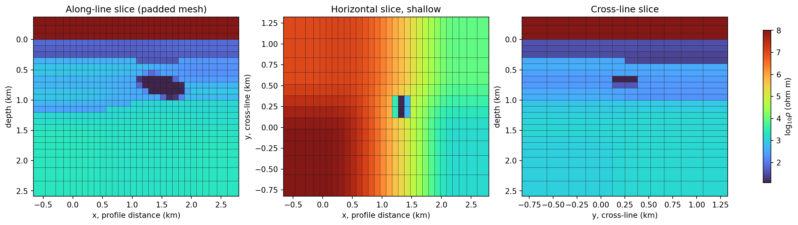
Mesh cell boundaries are drawn with pycsamt.api.mesh.draw_mesh() (preset="review") on every panel – the same reusable overlay used throughout this documentation, not something specific to this tutorial. The along-line slice (left) shows numerical air above the real terrain, the layered prior below it, and the seeded conductive lens as the dark patch near 1.3–1.7 km profile distance. The mesh stayed at 9,000 padded cells here, comfortably inside what the in-process solver can attempt – this section’s point is that a small 3-D problem runs at all, not a replay of a deliberately oversized mesh.

Run the fast integration training. This executes for real during this documentation build, on a training budget small enough to finish in a few minutes rather than hours:

>>> from pycsamt.agents import Inv3DAgent
>>> agent3d = Inv3DAgent(
...     physics="mt3d", n_layers=6,
...     freqs=np.geomspace(1.0, 1000.0, 8), depth_max=1800.0,
...     n_train_profiles=10, epochs=20, radius=450.0,
...     hidden=(64, 32), dropout=0.1, n_mc=0,
...     geology_grid_nx_ny=4, geology_grid_nz=4, max_mesh_cells=60_000,
... )
>>> res3d = agent3d.execute({
...     "sites": combined, "coords": coords, "topography": True,
...     "output_dir": "runs/willy_ai3d_maxwell",
... })
>>> res3d.status, res3d.data["pred_rho"].shape
('success', (50, 6))

Gate the result the same way as the 2-D section, before looking at the figure it produces:

>>> recovery3d = res3d.data["mt3d_recovery"]
>>> response_pass = res3d.data["rms_global"] <= 1.2
>>> recovery_pass = recovery3d["rmse"] <= 0.25 and recovery3d["r2"] >= 0.60
>>> enough_test_models = recovery3d["n_samples"] >= 20
>>> promote = response_pass and recovery_pass and enough_test_models
>>> promote
False

For the run captured on this page, rms_global was 2.244 and mt3d_recovery was {'rmse': 0.536, 'mae': 0.444, 'r2': -0.147, 'n_samples': 1} ((9) in AI inversion agents defines these). Both gates fail, as expected at this budget, and one held-out volume is far too few to trust r2’s sign. Re-running this exact call has already produced rms_global values from 1.5 to 6.5 across otherwise-identical seeded sessions on this machine – the same open reproducibility gap already documented for physics="mt1d" in AI inversion agents extends to the mt3d combined-line path too, since dataset realizations are seed-controlled but network initialization and dropout still consume PyTorch’s global random state. Treat any single captured RMS here as one draw, not a reproducible constant.

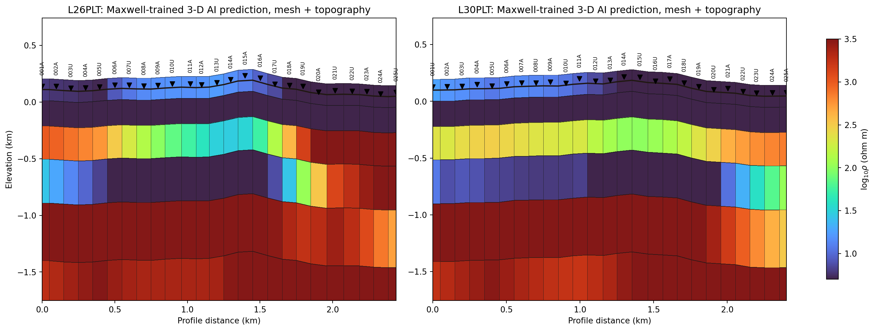
Each line’s own slice is cut from the single combined prediction – not two independent inversions – with the same station-index caution as before: never stitch L26PLT’s last station to L30PLT’s first as if adjacent. The mesh overlay makes the display grid’s actual cell resolution visible under the color, the black line is real station topography from pycsamt.topo.drape_section(), and triangles with rotated labels mark every station on both lines.

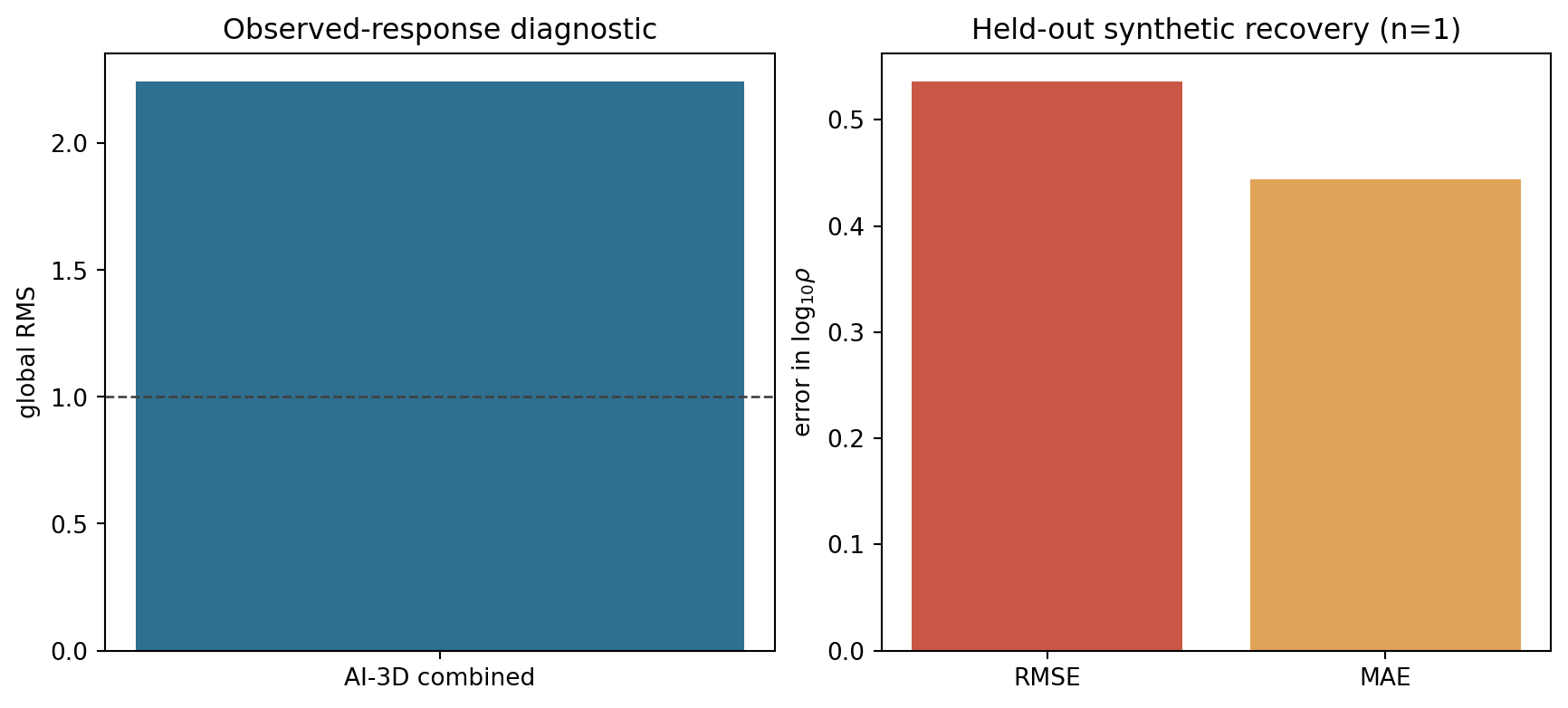
Both panels read the same way as the 2-D validation figure: the dashed line at RMS 1 is a rough response-fit reference, not a pass threshold on its own, and RMSE/MAE come from the single held-out volume discussed above.

Scale this up the same way the 2-D production configuration does – more realizations, more epochs, a finer geology grid – but budget accordingly. This project-scale configuration is deliberately not executed on this page; unlike the 2-D case, a realistic 3-D realization count on this survey is expected to take several hours to tens of hours on a single CPU core, not minutes:

>>> production_agent3d = Inv3DAgent(
...     physics="mt3d", n_layers=10,
...     freqs=np.geomspace(1.0, 10_000.0, 24), depth_max=2200.0,
...     n_train_profiles=200, epochs=60, radius=450.0,
...     hidden=(128, 64, 32), dropout=0.1, n_mc=0,
...     correlation_length_x_m=(300.0, 1200.0),
...     correlation_length_y_m=(300.0, 900.0),
...     correlation_length_z_m=(80.0, 400.0),
...     log_resistivity_mean=2.1, log_resistivity_std=0.75,
...     geology_grid_nx_ny=8, geology_grid_nz=8,
...     mesh_safety_factor=8.0, max_mesh_cells=300_000,
... )
>>> production_agent3d.physics, production_agent3d.n_train_profiles
('mt3d', 200)

Copy the complete pipeline – geology and mesh construction, the fast run, the production configuration, and every figure above – from the accordion below, and run it yourself for the full realization count:

</>View and copy the complete L26/L30 Maxwell 3-D AI workflowClick to inspect and copy the complete code

"""Run and plot the two-line Maxwell 3-D AI workflow used by the porphyry tutorial."""

from __future__ import annotations

import argparse
import json
import sys
import time
from pathlib import Path

import matplotlib

matplotlib.use("Agg")
import matplotlib.pyplot as plt
import numpy as np

ROOT = Path(__file__).resolve().parents[2]
sys.path.insert(0, str(ROOT))

from pycsamt.agents import Inv3DAgent  # noqa: E402
from pycsamt.ai.geology import (  # noqa: E402
    ElectricalLayer,
    EllipsoidalLens,
    GaussianCorrelation,
    GeologyGrid,
    generate_layered_geology,
    insert_lenses,
)
from pycsamt.api.mesh import PYCSAMT_MESH, cell_edges_from_centres, draw_mesh  # noqa: E402
from pycsamt.emtools import ensure_sites  # noqa: E402
from pycsamt.forward.maxwell import MeshDesign, build_solver_mesh  # noqa: E402
from pycsamt.topo import (  # noqa: E402
    drape_section,
    extract_chainage,
    extract_elevation,
    extract_station_names,
    interp_elev,
)

IMAGE_DIR = ROOT / "docs/source/images/tutorials/map_porphyry_mineralization_from_noisy_amt"
RUN_DIR = ROOT / "runs"

FAST_FREQUENCIES_HZ = np.geomspace(1.0, 1000.0, 8)
DEPTH_MAX_M = 1800.0
LINE_OFFSET_M = 500.0  # stated assumption: no real cross-line coordinate exists


def save(fig: plt.Figure, name: str) -> None:
    IMAGE_DIR.mkdir(parents=True, exist_ok=True)
    fig.savefig(IMAGE_DIR / name, dpi=190, bbox_inches="tight")
    plt.close(fig)


def load_lines():
    lines = {}
    for name in ("L26PLT", "L30PLT"):
        corrected = RUN_DIR / f"{name}_corrected"
        if not corrected.exists():
            raise FileNotFoundError(
                f"{corrected} is missing; run the tutorial's correction/export steps first."
            )
        lines[name] = ensure_sites(corrected, recursive=False, verbose=0).ordered()
    return lines


def build_combined_problem(lines):
    sites26, sites30 = lines["L26PLT"], lines["L30PLT"]
    chain26_m = extract_chainage(sites26) * 1000.0
    chain30_m = extract_chainage(sites30) * 1000.0
    coords = np.column_stack(
        [
            np.concatenate([chain26_m, chain30_m]),
            np.concatenate(
                [np.zeros_like(chain26_m), np.full_like(chain30_m, LINE_OFFSET_M)]
            ),
        ]
    )
    combined_sites = sites26.to_edis() + sites30.to_edis()

    x_span = float(coords[:, 0].max() - coords[:, 0].min())
    grid = GeologyGrid.regular_3d(
        nx=24,
        ny=6,
        nz=18,
        dx_m=x_span / 24.0,
        dy_m=(LINE_OFFSET_M + 300.0) / 6.0,
        dz_m=DEPTH_MAX_M / 18.0,
        x_origin_m=-150.0,
        y_origin_m=-150.0,
    )
    # A seeded display prior: this step is a mesh/geometry illustration only,
    # not the training distribution -- Inv3DAgent(physics="mt3d") builds its
    # own internal GeologyGrid from correlated fields; no agent constructor
    # accepts an externally-built grid.
    correlation = GaussianCorrelation(700.0, 160.0, length_y_m=500.0)
    layers = [
        ElectricalLayer("weathered cover", 45.0, 0.10, correlation),
        ElectricalLayer("altered intrusive", 350.0, 0.16, correlation),
        ElectricalLayer("fresh intrusive", 1600.0, 0.10, correlation),
    ]
    base = generate_layered_geology(
        grid, layers, [320.0, 1050.0], seed=2601,
        interface_relief_std_m=[45.0, 100.0],
        interface_correlation=correlation,
        minimum_thickness_m=120.0,
    )
    target = EllipsoidalLens(
        "combined-line conductive target",
        center_x_m=1500.0, center_y_m=LINE_OFFSET_M / 2.0, center_z_m=760.0,
        radius_x_m=480.0, radius_y_m=350.0, radius_z_m=210.0,
        resistivity_ohm_m=12.0, dip_deg=15.0, transition_fraction=0.20,
    )
    geology = insert_lenses(base, [target])
    solver_model = build_solver_mesh(
        grid,
        resistivity_ohm_m=geology.resistivity_ohm_m,
        frequencies_hz=FAST_FREQUENCIES_HZ,
        design=MeshDesign(
            horizontal_padding_cells=3,
            bottom_padding_cells=4,
            air_layers=3,
            padding_expansion=1.3,
        ),
    )
    return {
        "lines": lines,
        "sites26": sites26,
        "sites30": sites30,
        "chain26_m": chain26_m,
        "chain30_m": chain30_m,
        "coords": coords,
        "combined_sites": combined_sites,
        "grid": grid,
        "solver_model": solver_model,
    }


def plot_geology_and_mesh(problem) -> None:
    mesh_model = problem["solver_model"]
    centres = mesh_model.mesh.cell_centres_m
    x_km = centres["x"] / 1000.0
    y_km = centres["y"] / 1000.0
    z_km = centres["z"] / 1000.0
    x_edges = cell_edges_from_centres(x_km)
    y_edges = cell_edges_from_centres(y_km)
    z_edges = cell_edges_from_centres(z_km)
    log_rho = np.log10(1.0 / mesh_model.conductivity_s_m)
    mesh_style = PYCSAMT_MESH.style_for("review")
    fig, axes = plt.subplots(1, 3, figsize=(14.5, 4.0), constrained_layout=True)

    xz, _ = draw_mesh(
        axes[0], x_edges, z_edges, log_rho[:, log_rho.shape[1] // 2, :],
        style=mesh_style, cmap="turbo",
    )
    axes[0].invert_yaxis()
    axes[0].set(
        title="Along-line slice (padded mesh)",
        xlabel="x, profile distance (km)", ylabel="depth (km)",
    )

    draw_mesh(
        axes[1], x_edges, y_edges, log_rho[log_rho.shape[0] // 3, :, :],
        style=mesh_style, cmap="turbo",
    )
    axes[1].set(
        title="Horizontal slice, shallow",
        xlabel="x, profile distance (km)", ylabel="y, cross-line (km)",
    )

    draw_mesh(
        axes[2], y_edges, z_edges, log_rho[:, :, log_rho.shape[2] // 2],
        style=mesh_style, cmap="turbo",
    )
    axes[2].invert_yaxis()
    axes[2].set(
        title="Cross-line slice",
        xlabel="y, cross-line (km)", ylabel="depth (km)",
    )
    fig.colorbar(xz, ax=axes, shrink=0.85, label=r"$\log_{10}\rho$ (ohm m)")
    save(fig, "willy_ai3d_geology_maxwell_both_lines.png")


def run_fast_inversion(problem):
    np.random.seed(17)
    try:
        import torch

        torch.manual_seed(17)
    except ImportError:
        pass

    output_dir = RUN_DIR / "willy_ai3d_maxwell"
    output_dir.mkdir(parents=True, exist_ok=True)
    started = time.time()
    agent = Inv3DAgent(
        physics="mt3d",
        n_layers=6,
        freqs=FAST_FREQUENCIES_HZ,
        depth_max=DEPTH_MAX_M,
        n_train_profiles=10,
        epochs=20,
        radius=450.0,
        hidden=(64, 32),
        dropout=0.1,
        n_mc=0,
        geology_grid_nx_ny=4,
        geology_grid_nz=4,
        max_mesh_cells=60_000,
    )
    result = agent.execute(
        {
            "sites": problem["combined_sites"],
            "coords": problem["coords"],
            "topography": True,
            "output_dir": str(output_dir),
        }
    )
    if result.status != "success":
        raise RuntimeError(f"3-D fast run failed: {result.summary}")
    checkpoint = output_dir / "gcn_inverter_3d_maxwell.npz"
    result.data["inverter"].save(checkpoint)
    recovery = result.data.get("mt3d_recovery") or {}
    manifest = {
        "status": result.status,
        "summary": result.summary,
        "seed": 17,
        "n_train_profiles": 10,
        "epochs_requested": 20,
        "n_layers": 6,
        "depth_max_m": DEPTH_MAX_M,
        "line_offset_m": LINE_OFFSET_M,
        "frequencies_hz": FAST_FREQUENCIES_HZ.tolist(),
        "rms_global": float(result.data["rms_global"]),
        "mt3d_recovery": recovery,
        "elapsed_seconds": time.time() - started,
        "checkpoint": checkpoint.name,
    }
    (output_dir / "run_manifest.json").write_text(
        json.dumps(manifest, indent=2, default=float), encoding="utf-8"
    )
    print(json.dumps(manifest, default=float), flush=True)
    return result


def _cell_edges_km(centres_m: np.ndarray) -> np.ndarray:
    return cell_edges_from_centres(centres_m) / 1000.0


def plot_inversion_with_mesh(problem, result) -> None:
    pred_rho = np.asarray(result.data["pred_rho"], dtype=float)
    depths_km = np.asarray(result.data["depths_km"], dtype=float)
    n26 = len(problem["sites26"])
    pred26, pred30 = pred_rho[:n26], pred_rho[n26:]
    chain26_km = problem["chain26_m"] / 1000.0
    chain30_km = problem["chain30_m"] / 1000.0
    elev26 = extract_elevation(problem["sites26"])
    elev30 = extract_elevation(problem["sites30"])
    labels26 = [n.split("-")[-1] for n in extract_station_names(problem["sites26"])]
    labels30 = [n.split("-")[-1] for n in extract_station_names(problem["sites30"])]
    z_edges_km = cell_edges_from_centres(depths_km)

    fig, axes = plt.subplots(1, 2, figsize=(15.0, 5.6), constrained_layout=True)
    mesh_style = PYCSAMT_MESH.style_for("review")
    fills = []
    for ax, chain_km, elev_m, labels, pred, name in zip(
        axes,
        (chain26_km, chain30_km),
        (elev26, elev30),
        (labels26, labels30),
        (pred26, pred30),
        ("L26PLT", "L30PLT"),
    ):
        x_edges_km = cell_edges_from_centres(chain_km)
        x_centres = 0.5 * (x_edges_km[:-1] + x_edges_km[1:])
        elev_centres_km = interp_elev(chain_km, elev_m / 1000.0, x_centres)
        data = pred.T  # (n_layers, n_sta)
        x_nodes, z_draped, data_draped = drape_section(
            x_edges_km, z_edges_km, data, elev_centres_km
        )
        x_2d = np.broadcast_to(x_nodes[None, :], z_draped.shape)
        fill, _edges = draw_mesh(
            ax, x_2d, z_draped, data_draped, style=mesh_style,
            cmap="turbo", vmin=0.7, vmax=3.5,
        )
        fills.append(fill)
        surface_km = interp_elev(chain_km, elev_m / 1000.0, x_nodes)
        ax.plot(x_nodes, surface_km, color="#211813", linewidth=1.6, zorder=8)
        marker_y = elev_m / 1000.0 + 0.03
        ax.scatter(chain_km, marker_y, marker="v", s=32, color="black", zorder=10)
        for xi, yi, lab in zip(chain_km, marker_y + 0.10, labels):
            ax.text(
                xi, yi, lab, rotation=90, ha="center", va="bottom",
                fontsize=6.6, zorder=11,
            )
        ax.set_ylim(float(surface_km.min() - depths_km[-1]), float(surface_km.max() + 0.55))
        ax.set_xlim(float(chain_km.min()), float(chain_km.max()))
        ax.set_xlabel("Profile distance (km)")
        ax.set_title(f"{name}: Maxwell-trained 3-D AI prediction, mesh + topography")
    axes[0].set_ylabel("Elevation (km)")
    fig.colorbar(fills[0], ax=axes, label=r"$\log_{10}\rho$ (ohm m)", shrink=0.85)
    save(fig, "willy_ai3d_maxwell_predictions_both_lines.png")


def plot_validation(result) -> None:
    recovery = result.data.get("mt3d_recovery") or {}
    fig, axes = plt.subplots(1, 2, figsize=(9.0, 4.0), constrained_layout=True)
    axes[0].bar(["AI-3D combined"], [float(result.data["rms_global"])], color="#2f6f8f")
    axes[0].axhline(1, color="0.25", ls="--", lw=1)
    axes[0].set(title="Observed-response diagnostic", ylabel="global RMS")
    axes[1].bar(
        ["RMSE", "MAE"],
        [float(recovery.get("rmse", np.nan)), float(recovery.get("mae", np.nan))],
        color=["#c85745", "#e0a458"],
    )
    axes[1].set(
        title=f"Held-out synthetic recovery (n={recovery.get('n_samples', 0)})",
        ylabel=r"error in $\log_{10}\rho$",
    )
    save(fig, "willy_ai3d_maxwell_validation_both_lines.png")


def production_config_reference():
    """Configuration-only reference for a real, many-hour 3-D run.

    Not executed here. Copy this function's body (or run this script with
    ``--production``) in your own environment; a realistic budget for this
    survey is likely several hours to tens of hours on a single CPU core,
    depending on ``n_train_profiles``, ``geology_grid_nx_ny/nz``, and
    ``max_mesh_cells``.
    """
    return Inv3DAgent(
        physics="mt3d",
        n_layers=10,
        freqs=np.geomspace(1.0, 10_000.0, 24),
        depth_max=2200.0,
        n_train_profiles=200,
        epochs=60,
        radius=450.0,
        hidden=(128, 64, 32),
        dropout=0.1,
        n_mc=0,
        correlation_length_x_m=(300.0, 1200.0),
        correlation_length_y_m=(300.0, 900.0),
        correlation_length_z_m=(80.0, 400.0),
        log_resistivity_mean=2.1,
        log_resistivity_std=0.75,
        geology_grid_nx_ny=8,
        geology_grid_nz=8,
        mesh_safety_factor=8.0,
        max_mesh_cells=300_000,
    )


def main(argv: list[str] | None = None) -> int:
    parser = argparse.ArgumentParser()
    parser.add_argument(
        "--production",
        action="store_true",
        help="Build the production agent (configuration only; does NOT execute).",
    )
    args = parser.parse_args(argv)

    lines = load_lines()
    problem = build_combined_problem(lines)
    plot_geology_and_mesh(problem)

    if args.production:
        agent = production_config_reference()
        print(
            "production config only, not executed:",
            agent.physics, agent.n_train_profiles, agent.epochs,
        )
        return 0

    result = run_fast_inversion(problem)
    plot_inversion_with_mesh(problem, result)
    plot_validation(result)

    quality = problem["solver_model"].quality
    recovery = result.data.get("mt3d_recovery") or {}
    print(
        "combined",
        "stations", len(problem["combined_sites"]),
        "geology", problem["grid"].shape,
        "mesh", problem["solver_model"].mesh.shape,
        "cells", quality.cell_count,
        "RMS", f"{result.data['rms_global']:.3f}",
        "recovery_RMSE", f"{recovery.get('rmse', float('nan')):.3f}",
        "recovery_n", recovery.get("n_samples", 0),
    )
    return 0


if __name__ == "__main__":
    raise SystemExit(main())

Run it after the corrected EDI export step, exactly like the 2-D script:

python docs/scripts/generate_tutorial_porphyry_ai3d_workflow.py

Executed output:

combined stations 50 geology (18, 6, 24) mesh (25, 12, 30) cells 9000 RMS 2.244 recovery_RMSE 0.536 recovery_n 1

Pass --production to build (but not execute) the production agent instead of running the fast one – it prints its configuration and returns without training, so you can inspect the object before committing CPU time:

python docs/scripts/generate_tutorial_porphyry_ai3d_workflow.py --production

18.16.19. Correction Parameter Report

A production project should archive, per station, exactly what was decided and why. Build one table per line from the intermediate results already computed above.

>>> import pandas as pd
>>> pd.set_option("display.width", 160)
>>> pd.set_option("display.max_columns", None)
>>> report26 = gb26[["station", "gain", "twist_deg", "shear"]].merge(
...     ns26[["station", "ns_index", "ss_delta_log10", "distortion_type"]], on="station", how="left"
... ).merge(
...     factors26[["station", "fac_z_reviewed"]], on="station", how="left"
... )
>>> report26["strike_deg"] = -36.42
>>> report26["emap_method"] = "flma"
>>> report26.iloc[[0, 15, 19, 20]].round(3)
    station  gain  twist_deg  shear  ns_index  ss_delta_log10 distortion_type  fac_z_reviewed  strike_deg emap_method
0   26-001A   1.0     19.724 -0.466     1.625           0.496          static           0.565      -36.42        flma
15  26-016A   1.0     -0.505  0.175     1.907           0.151          static           0.840      -36.42        flma
19  26-020A   1.0     60.352  0.544     2.378           0.667           mixed           0.464      -36.42        flma
20  26-021U   1.0    -14.728  0.891     1.244          -0.647          static           2.107      -36.42        flma

>>> report26["distortion_type"].value_counts().to_dict()
{'mixed': 17, 'static': 8}
>>> round(report26["twist_deg"].abs().median(), 2), round(report26["fac_z_reviewed"].median(), 3)
(8.34, 0.542)

>>> report30 = gb30[["station", "gain", "twist_deg", "shear"]].merge(
...     ns30[["station", "ns_index", "ss_delta_log10", "distortion_type"]], on="station", how="left"
... ).merge(
...     factors30[["station", "fac_z_reviewed"]], on="station", how="left"
... )
>>> report30["strike_deg"] = -45.84
>>> report30["emap_method"] = "flma"
>>> report30["distortion_type"].value_counts().to_dict()
{'static': 13, 'mixed': 12}
>>> round(report30["twist_deg"].abs().median(), 2), round(report30["fac_z_reviewed"].median(), 3)
(10.37, 0.535)

Save both tables next to the corrected EDIs so a reviewer – or a future run of this same pipeline – can see exactly which correction each station received without re-deriving it:

>>> report26.to_csv("runs/L26PLT_correction_report.csv", index=False)
>>> report30.to_csv("runs/L30PLT_correction_report.csv", index=False)

18.16.20. Adapting This Tutorial

For a different two-line project, change only the input folders first:

line_a_dir = "path/to/your/line_a_edis"
line_b_dir = "path/to/your/line_b_edis"

Then rerun the same sequence. If your survey has tipper, add it to the strike and rotation sections following Condition an MT Line With Tipper and Rotation. If the strike rose is tight rather than broad, trust the rotation more; if it is broad like both lines here, retain the full tensor for an external 3-D Maxwell inversion rather than treating the station-graph candidate as a physical cross-check. If your survey does have a real controlled-source transmitter, Map Groundwater Geology From CSAMT covers the near-field and source-overprint diagnostics this tutorial deliberately omits.

18.16.21. See Also

Correct Static Shift

A single-line, single-method static-shift workflow to compare against the conditional approach used here.

Condition an MT Line With Tipper and Rotation

The nearest existing precedent for the QC-to-rotation portion of this workflow, on a quieter MT line with tipper.

Prepare an Occam2D Inversion

The Occam2D preparation pattern reused above, in full single-line depth.

Run Classical Inversions: Occam2D, ModEM, and MARE2DEM

How to locate or build the Occam2D/ModEM binaries, launch the runs prepared above, and load the results.

Building a Defensible 3-D AI Inversion Problem

Construction and capability gating for a genuine topographic 3-D geology and Maxwell problem.

Map Groundwater Geology From CSAMT

The near-field and source-overprint diagnostics this tutorial omits, run for real against a real ten-station CSAMT line.

Field Zones: Near, Transition, And Far Field

The full near-field and source-overprint theory behind that companion tutorial’s diagnostics.

Static Shift

The physics and correction-factor derivation behind the static-shift section.

ModEM

Full ModEM backend documentation.

Choosing A Model Backend

Deciding between Occam2D, ModEM, MARE2DEM, and AI inversion.