
11.7. Phase Tensor And Impedance Tensor Tools#
The tensor page is one of the central pages in the pyCSAMT user guide
because it connects interpretation and preprocessing. The same
impedance tensor Z supports apparent resistivity, phase,
skew, geoelectric strike, static-shift checks, dimensionality
checks, and 2-D rotation decisions. The pycsamt.emtools tensor
tools expose two main workflows:
Workflow |
Main tools |
Purpose |
|---|---|---|
Phase-tensor interpretation |
|
Diagnose dimensionality, strike, skew, ellipticity, and spatial coherence without being dominated by static-shift amplitude. |
Impedance-tensor editing |
|
Apply deliberate preprocessing operations to |
The phase tensor follows the Caldwell, Bibby & Brown (2004) decomposition. For each frequency, pyCSAMT splits the impedance tensor into real and imaginary parts, then computes the phase tensor and its invariants. Writing
the phase tensor is
If \(X\) is singular, pyCSAMT falls back to a pseudo-inverse. The important interpretation point is that \(\Phi\) is built from a ratio of the imaginary and real impedance parts. A real, frequency independent static shift multiplier scales \(X\) and \(Y\) together, so it largely cancels in \(X^{-1}Y\). That is why phase tensor plots are such useful companions to apparent-resistivity and static-shift diagnostics.
The examples in this guide use public two-level imports from
pycsamt.emtools. One name needs special attention:
pycsamt.emtools.rotate_to_strike belongs to the strike module, while
the tensor module’s own strike rotation helper is exported as
rotate_z_to_strike.
11.7.1. Load Data#
Start with the canonical loader. It returns a Sites object and skips
stations without valid impedance data.
>>> from pathlib import Path
>>> from pycsamt.emtools import ensure_sites
>>> edi_dir = Path("data/AMT/WILLY_DATA/L18PLT")
>>> sites = ensure_sites(
...     edi_dir,
...     recursive=True,
...     on_dup="replace",
...     strict=False,
...     verbose=0,
... )
Keep sites as the unmodified reference object. Tensor editing
functions can return corrected copies when inplace=False, so it is
easy to compare original and edited data.
11.7.2. Build The Phase-Tensor Table#
build_phase_tensor_table is the foundation for the plotting tools.
It returns one row per station and frequency. For a phase tensor
pyCSAMT reports the Caldwell-style angles
using atan2 internally so the quadrant is preserved. The table
stores beta again as skew. These two angles play very different
roles: \(\alpha\) shifts whenever the coordinate frame is rotated –
it behaves like an ordinary strike angle – while \(\beta\) is
provably invariant under coordinate rotation, which is exactly what
makes skew usable as a distortion and dimensionality diagnostic
rather than just another orientation number. The “Audit Edits With
Phase-Tensor Tables” section later on this page demonstrates that
invariance directly on real data: rotating every station by a fixed
angle changes theta but leaves skew completely unchanged.
The principal values \(\phi_{\max}\) and \(\phi_{\min}\) are the
singular values of \(\Phi\); these appear in the table as s1 and
s2. The ellipse orientation theta is the angle of the dominant
left singular vector. Since an ellipse has no arrow head, theta is
axial: \(\theta\) and \(\theta+180^\circ\) describe the same
direction.
The ellipticity is
Values near zero are close to circular. Larger values mean the tensor has a stronger preferred axis, but that axis should still be read together with skew and period stability.
>>> from pycsamt.emtools import build_phase_tensor_table
>>> pt = build_phase_tensor_table(
...     sites,
...     recursive=False,
... )
>>> print(pt.head())
   station     freq    period  ...      beta      skew    ellipt
0  18-001A  10400.0  0.000096  ...  2.611588  2.611588  0.194909
1  18-001A   8707.0  0.000115  ...  1.964321  1.964321  0.210163
2  18-001A   7289.0  0.000137  ...  1.804266  1.804266  0.213894
3  18-001A   6102.0  0.000164  ...  1.068855  1.068855  0.212655
4  18-001A   5108.0  0.000196  ... -6.949269 -6.949269  0.425503

[5 rows x 10 columns]
>>> print(pt[["station", "freq", "period", "theta", "skew", "ellipt"]])
      station       freq    period       theta       skew    ellipt
0     18-001A  10400.000  0.000096  120.687698   2.611588  0.194909
1     18-001A   8707.000  0.000115  123.342495   1.964321  0.210163
2     18-001A   7289.000  0.000137  126.743525   1.804266  0.213894
3     18-001A   6102.000  0.000164  116.947420   1.068855  0.212655
4     18-001A   5108.000  0.000196  126.074830  -6.949269  0.425503
...       ...        ...       ...         ...        ...       ...
1479  18-025A      2.052  0.487329  -34.147397 -20.351504  0.559680
1480  18-025A      1.718  0.582072    4.537986 -46.015322  0.196258
1481  18-025A      1.438  0.695410   40.621212 -73.461943  0.216635
1482  18-025A      1.204  0.830565 -125.802958 -87.940352  0.527659
1483  18-025A      1.008  0.992063 -107.576221  86.240927  0.931748

[1484 rows x 6 columns]
The table contains these core columns:
Column |
Meaning |
|---|---|
|
Station identifier. |
|
Frequency in hertz. |
|
Period in seconds, computed as |
|
Phase-tensor principal values. They control ellipse major and minor axes. |
|
Principal-axis angle, interpreted as phase-tensor strike. It is axial, so directions separated by 180 degrees are equivalent. |
|
Phase-tensor coordinate angle. Rotation-variant. |
|
Skew angle. |
|
Ellipticity, computed from the principal values. Values near zero are closer to circular; larger values indicate stronger 2-D anisotropy of the phase tensor. |
The table is also the best place to audit a survey numerically before plotting:
>>> summary = pt.groupby("station").agg(
...     n=("freq", "count"),
...     median_abs_skew=("skew", lambda values: values.abs().median()),
...     median_ellipt=("ellipt", "median"),
...     theta_iqr=("theta", lambda values: values.quantile(0.75) - values.quantile(0.25)),
... )
>>> print(summary.sort_values("median_abs_skew", ascending=False))
          n  median_abs_skew  median_ellipt   theta_iqr
station
18-023A  53        54.529465       0.776955  332.406202
18-022U  53        49.751057       0.765743  330.236042
18-021B  53        47.235914       0.917700   65.673584
18-021U  53        46.582007       0.975587    5.728713
18-020A  53        45.539049       0.890491    7.151592
18-018A  53        37.183191       0.747821   19.123004
18-022V  53        36.986632       0.734789   33.283984
18-019U  53        33.778453       0.610832   44.257571
18-025A  53        24.634843       0.666770  174.077409
18-017U  53        19.002375       0.660533  269.958366
18-023V  53        14.611436       0.568990   39.420996
18-014A  53        14.548260       0.735137  273.677122
18-004A  53        14.509282       0.683143   18.628263
18-015U  53        14.242493       0.721964  316.822496
18-009A  53        13.024178       0.477635   19.936171
18-006A  53        12.375357       0.574245   24.700266
18-016A  53        12.121341       0.732322  302.853539
18-013U  53        12.025504       0.591064   41.602228
18-024U  53        11.482211       0.696343   69.080189
18-003A  53        11.018588       0.674498   23.567376
18-011A  53         9.310687       0.692296  261.601465
18-010U  53         9.242375       0.676668  257.925336
18-005U  53         9.171151       0.598509   16.449050
18-008U  53         9.136982       0.459678   30.040274
18-012A  53         9.052529       0.710183   37.311060
18-007U  53         8.377503       0.492508   29.303937
18-002U  53         6.596544       0.535202   16.329767
18-001A  53         4.809977       0.423331   15.689190
Large median_abs_skew means the station is not behaving like a clean
1-D or 2-D response in that period range. Large theta_iqr means
phase-tensor strike changes strongly with frequency, so one rotation
angle may be a poor summary. With the corrected skew formula every
station in this survey now sits under a median absolute skew of 55
degrees – a very different, much more legible picture than a swapped
formula would produce, and one where several stations (18-001A,
18-002U, 18-005U through 18-012A) sit comfortably under
10 degrees.
11.7.3. Filter By Period#
Most tensor interpretation should be tied to a period band. A shallow band and a deeper band can show different strike, skew, or ellipticity.
>>> period_band = (0.001, 10.0)
>>> band_pt = pt[
...     (pt["period"] >= period_band[0])
...     & (pt["period"] <= period_band[1])
... ]
>>> print("rows in band:", len(band_pt))
rows in band: 1092
>>> print("stations in band:", band_pt["station"].nunique())
stations in band: 28
>>> print("median |skew|:", band_pt["skew"].abs().median())
median |skew|: 16.941088508206953
When you report a tensor result, always report the period band. A map at
period=1.0 second and a summary over 0.001 to 10.0 seconds
answer different questions.
11.7.4. Read Dimensionality From Skew And Ellipticity#
A simple phase-tensor dimensionality rule uses skew and ellipticity:
Class |
Rule |
Interpretation |
|---|---|---|
1-D |
|
Low skew and nearly circular phase tensor. |
2-D |
|
Low skew but elongated phase tensor. |
3-D |
|
High skew; strike and 2-D rotation should be treated with caution. |
>>> import numpy as np
>>> skew_threshold = 3.0
>>> ellipt_threshold = 0.2
>>> work = band_pt.copy()
>>> abs_skew = work["skew"].abs()
>>> abs_ellipt = work["ellipt"].abs()
>>> work["dimensionality"] = np.select(
...     [
...         (abs_skew <= skew_threshold) & (abs_ellipt <= ellipt_threshold),
...         (abs_skew <= skew_threshold) & (abs_ellipt > ellipt_threshold),
...     ],
...     ["1D", "2D"],
...     default="3D",
... )
>>> print(work["dimensionality"].value_counts(normalize=True))
dimensionality
3D    0.894689
2D    0.087912
1D    0.017399
Name: proportion, dtype: float64
The default 3 degree skew threshold is strict. It is useful as a
textbook 1-D/2-D screen, but it still classifies most real field samples
as 3-D here. That is not a failure of the function; it is a warning
about the data and the 2-D assumption. Note the scale of this number
compared to a swapped-formula run: with the correct, rotation-invariant
skew this survey classifies as roughly 90 percent 3-D rather than
the 97.5 percent an incorrect formula would have reported – the
threshold and the interpretation habit matter, but so does the sign and
identity of the quantity being thresholded.
In compact notation, the rule used by the example is
where \(\beta_0\) is skew_threshold and \(e_0\) is
ellipt_threshold. The threshold is a decision rule, not a law of
nature. For a field survey, report the threshold and the period band
with the result.
11.7.5. Simple Phase-Tensor Views#
Use the simpler plots before the full ellipse plot. They make it easy to identify which invariant is causing the interpretation.
View the executed simple-views source codeClick to inspect and copy the complete code
 1def make_simple_views_bundle() -> None:
 2    """Write the five quick-look diagnostic figures used by the "Simple
 3    Phase-Tensor Views" section: strike scatter, skew and ellipticity
 4    heatmaps, and the two dimensionality classifications.
 5    """
 6    sites = ensure_sites(L18PLT, recursive=True)
 7
 8    plot_theta_vs_period(sites, recursive=False)
 9    plt.gcf().savefig(IMAGES / "user-guide-emtools-tensor-06-01.png", dpi=200, bbox_inches="tight")
10    plt.close()
11
12    plot_phase_tensor_skewmap(sites, recursive=False, axis_y="logperiod")
13    plt.gcf().savefig(IMAGES / "user-guide-emtools-tensor-06-02.png", dpi=200, bbox_inches="tight")
14    plt.close()
15
16    plot_ellipticity_psection(sites, recursive=False)
17    plt.gcf().savefig(IMAGES / "user-guide-emtools-tensor-06-03.png", dpi=200, bbox_inches="tight")
18    plt.close()
19
20    plot_dimensionality_psection(
21        sites,
22        skew_th=3.0,
23        ellipt_th=0.2,
24        recursive=False,
25    )
26    plt.gcf().savefig(IMAGES / "user-guide-emtools-tensor-06-04.png", dpi=200, bbox_inches="tight")
27    plt.close()
28
29    plot_dimensionality_grid(
30        sites,
31        skew_th=3.0,
32        ellipt_th=0.2,
33        recursive=False,
34    )
35    plt.gcf().savefig(IMAGES / "user-guide-emtools-tensor-06-05.png", dpi=200, bbox_inches="tight")
36    plt.close()
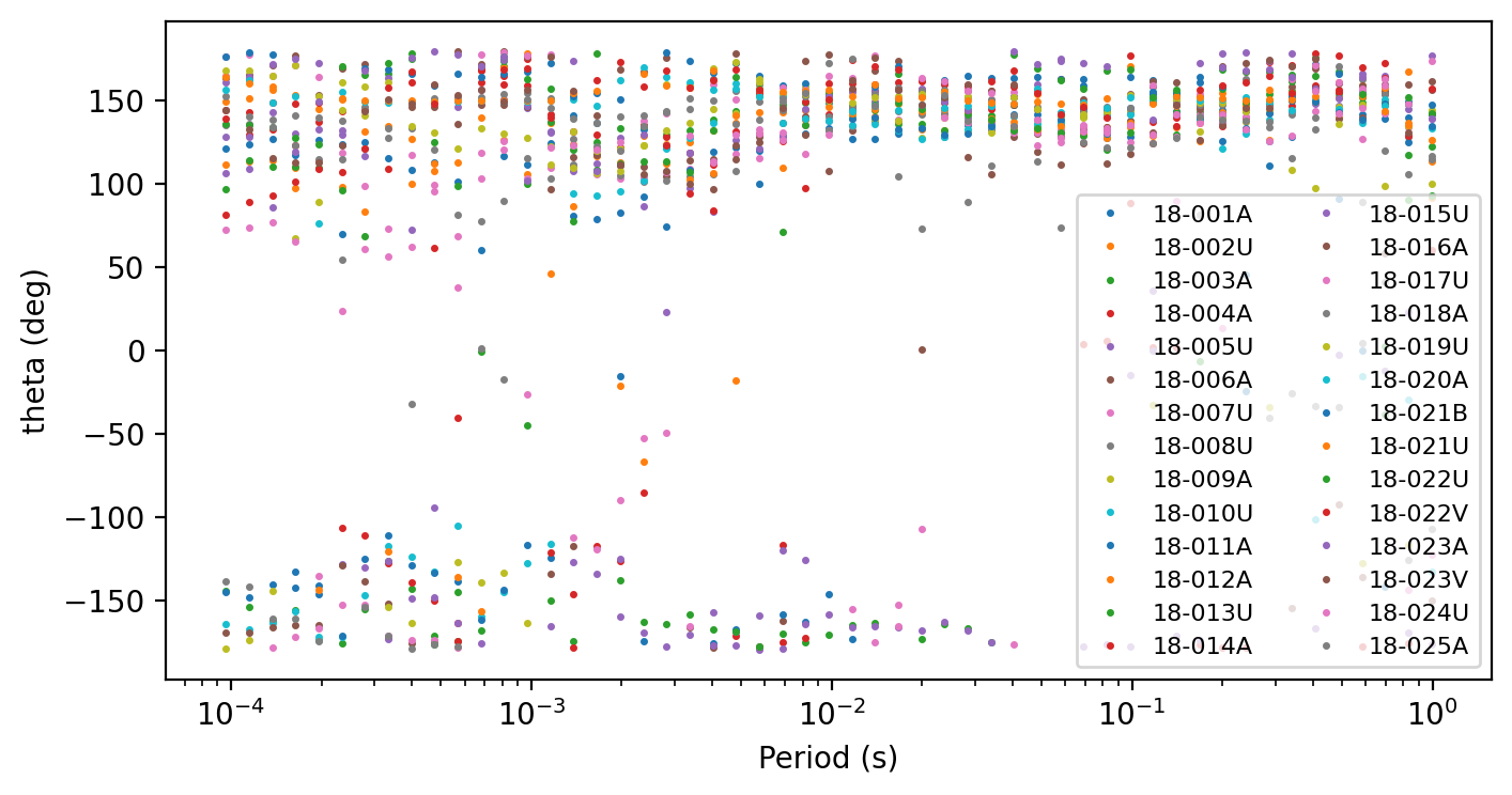
plot_theta_vs_period is a scatter view of strike angle by period.
It is quick, but it puts an axial angle on a linear y-axis. Treat jumps
near the wrap boundary carefully.
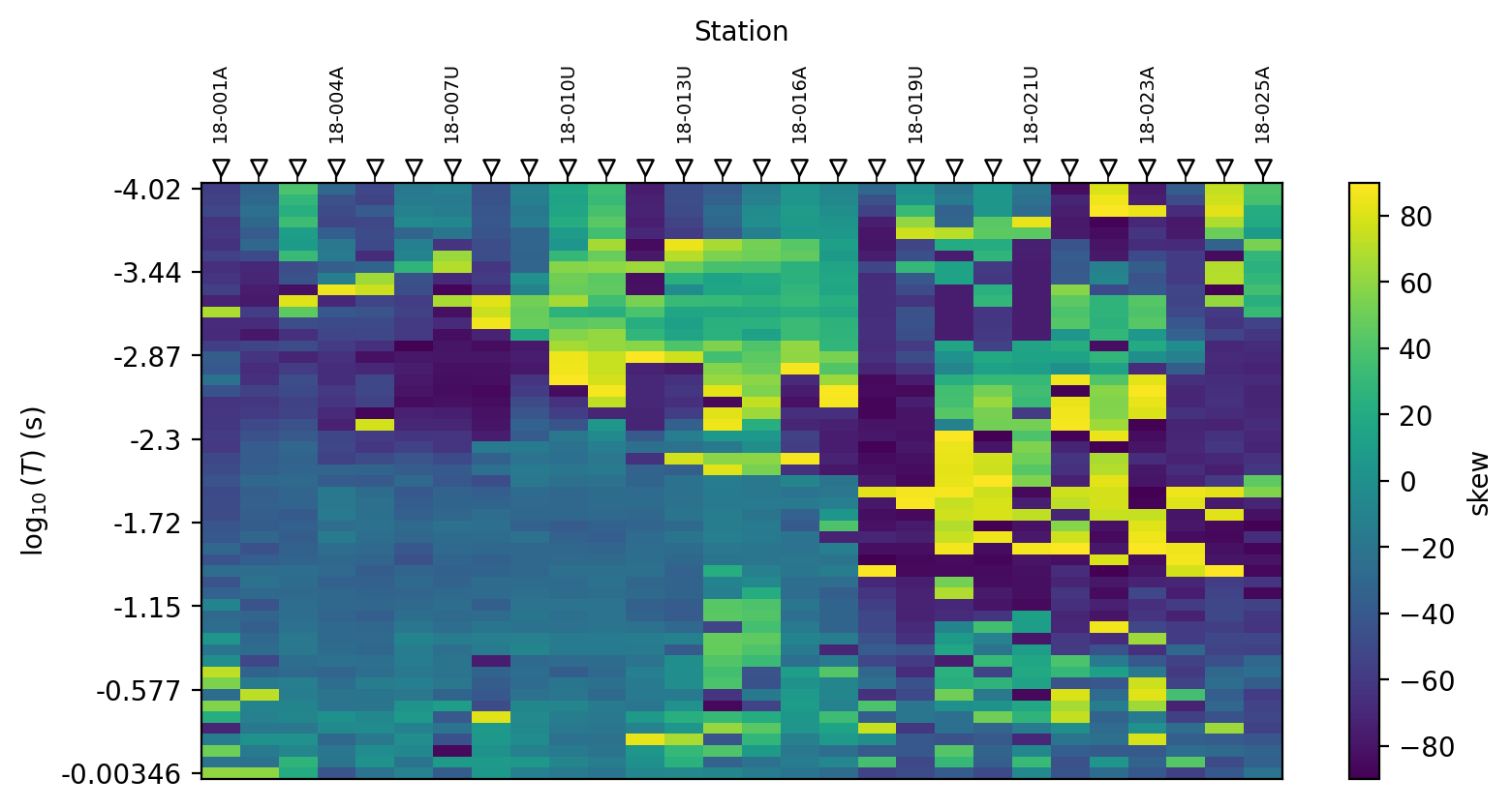
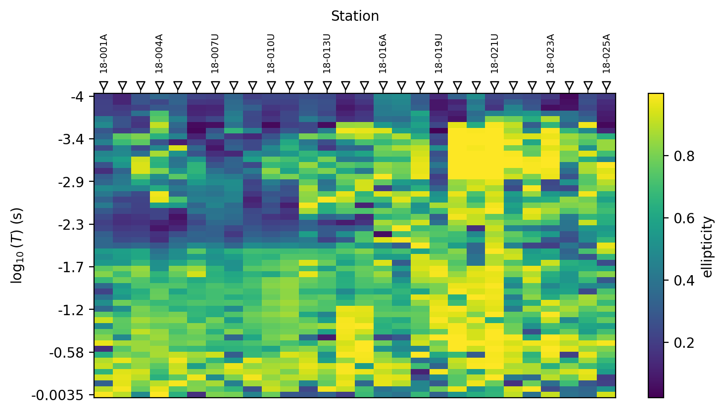
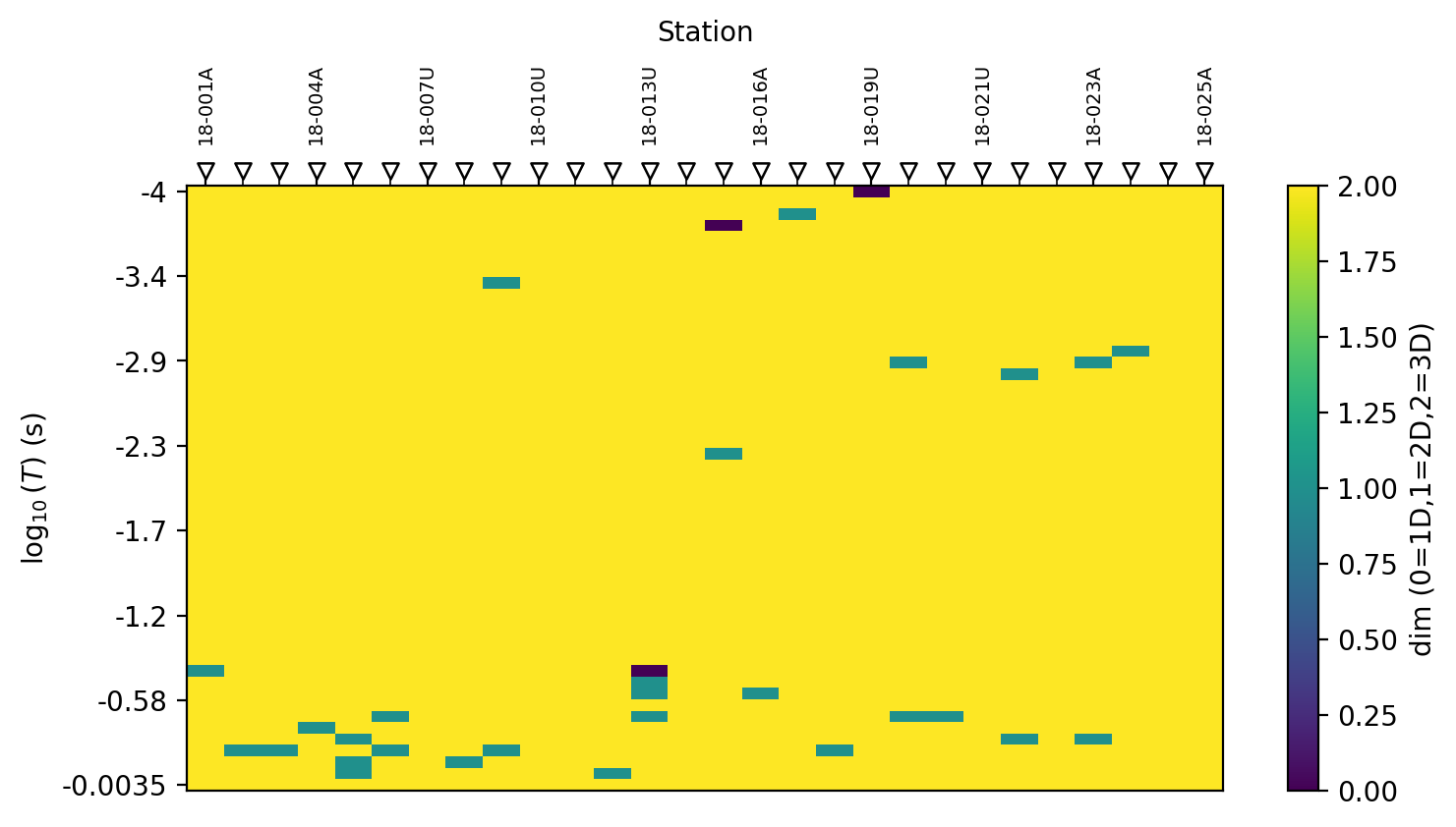
plot_phase_tensor_skewmap and plot_ellipticity_psection show
station-by-period heatmaps. They are good for finding period bands that
are consistently low-skew or strongly elongated.
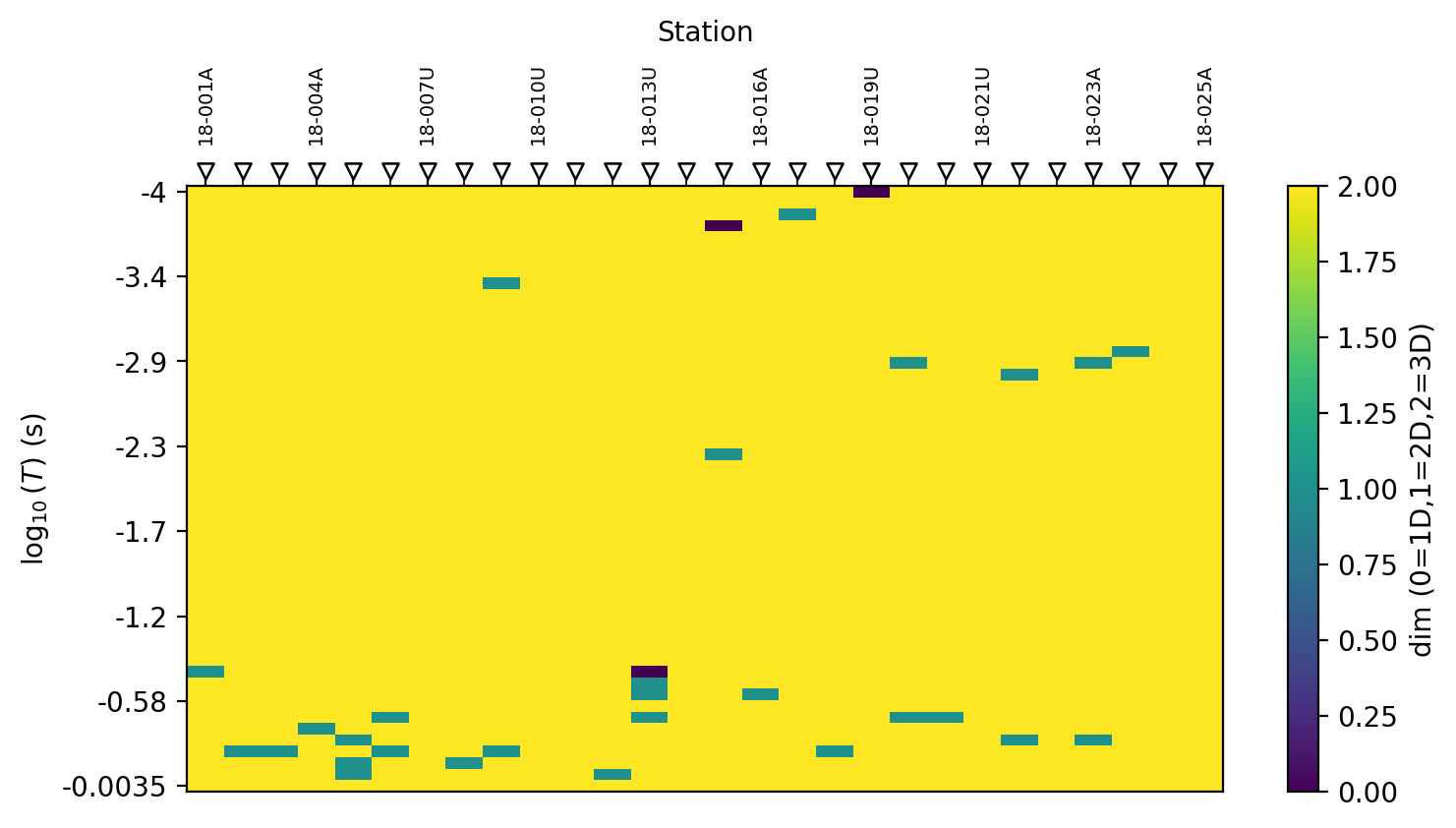
plot_dimensionality_psection and plot_dimensionality_grid apply
the simple skew/ellipticity classification to every station-period cell.
Read them alongside the table above: most of both panels should read
“3-D” at this survey’s default threshold, and that is expected given the
0.89 proportion computed numerically a moment ago, not a sign that
the plot is broken.
11.7.6. Phase-Tensor Ellipse Pseudosection#
plot_phase_tensor_psection is the main phase-tensor figure. Each
cell is an ellipse:
Visual element |
Meaning |
|---|---|
Major axis |
|
Minor axis |
|
Orientation |
|
Fill color |
Controlled by |
Thick border |
Optional marker for cells where |
>>> import matplotlib.pyplot as plt
>>> from pycsamt.emtools import plot_phase_tensor_psection
>>> _ = plot_phase_tensor_psection(
...     sites,
...     stations=None,
...     period_range=(0.001, 10.0),
...     axis_y="logperiod",
...     period_up=True,
...     c_by="skew",
...     skew_threshold=3.0,
...     mark_3d=True,
...     normalise_by="cell",
...     recursive=False,
... )
>>> plt.gcf().savefig(
...     "tensor_phase_tensor_psection.png",
...     dpi=200,
...     bbox_inches="tight",
... )
>>> plt.close()
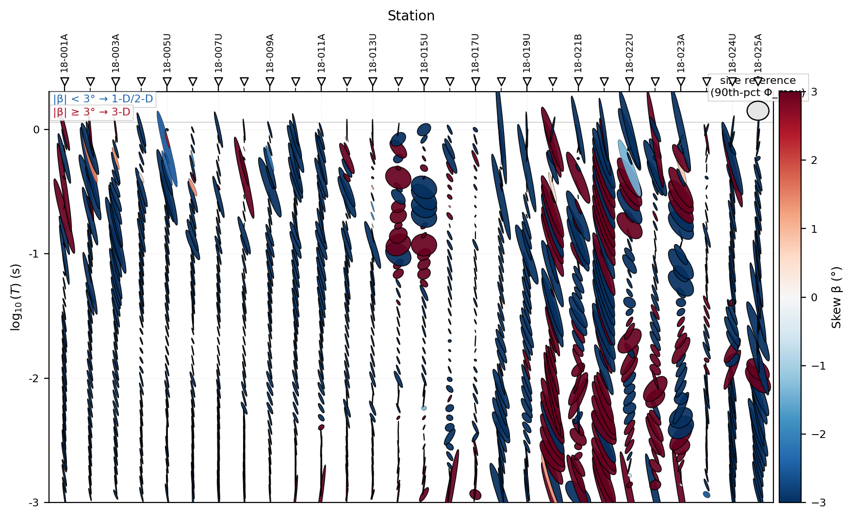
Most stations show thin, elongated slivers at short period (top of the
plot) that broaden and pick up stronger red/blue fill color at longer
period – the same short-period-cleaner, long-period-noisier pattern the
skew table already hinted at through low median values for stations like
18-001A and 18-002U. Useful c_by values include
"skew", "beta", "theta", "ellipt", "s1", "s2",
"|skew|", "phi_mean", "phi_max", and "phi_min".
Use normalise_by="cell" for most survey plots because it scales the
ellipses to the local plotting grid. Use normalise_by="unity" when
you want the 45-degree, 1-D reference to have an explicit visual meaning.
Use normalise_by="abs" only when absolute ellipse sizes in data units
are intentional.
The ellipse drawn at a station-period cell has semi-axes proportional to \(\phi_{\max}\) and \(\phi_{\min}\) and is rotated by \(\theta\). In local plot coordinates, before normalization, the ellipse satisfies
where
Changing normalise_by changes how those axes are scaled for display;
it does not change the phase-tensor values in the table.
11.7.7. A Full Tensor Is Not Optional#
Every formula above assumes a genuine \(2\times2\) impedance tensor
with independent Zxy and Zyx information. data/CSAMT is a
real, single-component Tongkeng CSAMT line – only Zxy is populated,
Zyx is identically zero – and it is a useful, real way to see what
happens when that assumption breaks.
>>> csamt = ensure_sites("data/CSAMT", recursive=False, verbose=0)
>>> pt_csamt = build_phase_tensor_table(csamt, recursive=False)
>>> print(pt_csamt.shape)
(170, 10)
>>> print(pt_csamt[["station", "freq", "s1", "s2", "theta", "skew", "ellipt"]].head(8))
  station        freq        s1   s2  theta  skew  ellipt
0  csa000  8196.72200  0.656877  0.0   90.0  90.0     1.0
1  csa000  4098.36100  0.216208  0.0   90.0  90.0     1.0
2  csa000  2049.18000  0.472698  0.0   90.0  90.0     1.0
3  csa000  1023.54100  0.340428  0.0   90.0   0.0     1.0
4  csa000   512.82060  0.218035  0.0   90.0   0.0     1.0
5  csa000   255.75450  0.002304  0.0   90.0  90.0     1.0
6  csa000   128.04100  0.044885  0.0   90.0   0.0     1.0
7  csa000    64.10257  0.170754  0.0   90.0   0.0     1.0
>>> print(pt_csamt[["theta", "skew", "ellipt", "s1", "s2"]].describe())
       theta        skew        ellipt          s1     s2
count  170.0  170.000000  1.700000e+02  170.000000  170.0
mean    90.0   23.823529  1.000000e+00    0.265513    0.0
std      0.0   39.823182  5.530282e-11    0.300118    0.0
min     90.0    0.000000  1.000000e+00    0.002304    0.0
25%     90.0    0.000000  1.000000e+00    0.080678    0.0
50%     90.0    0.000000  1.000000e+00    0.181731    0.0
75%     90.0   90.000000  1.000000e+00    0.319169    0.0
max     90.0   90.000000  1.000000e+00    2.390577    0.0
Every number here is a mathematical artifact, not geology. With
Zyx = 0 the phase tensor is exactly singular: s2 is zero at
every frequency and station (std is 0.0), so ellipt is
pinned at exactly 1.0 and theta is pinned at exactly 90
degrees regardless of what the earth is doing. skew does not settle
either – it alternates rigidly between 0 and 90 degrees as
atan2 picks a branch for a matrix entry that is exactly zero. Seeing
the same rigid pattern in a real pseudosection makes this concrete:
>>> _ = plot_phase_tensor_psection(
...     csamt,
...     stations=None,
...     axis_y="logperiod",
...     period_up=True,
...     c_by="skew",
...     skew_threshold=3.0,
...     mark_3d=True,
...     normalise_by="cell",
...     recursive=False,
...     title="CSAMT (single-component Zxy): degenerate phase tensor",
... )
>>> plt.gcf().savefig("tensor_csamt_degenerate.png", dpi=200, bbox_inches="tight")
>>> plt.close()
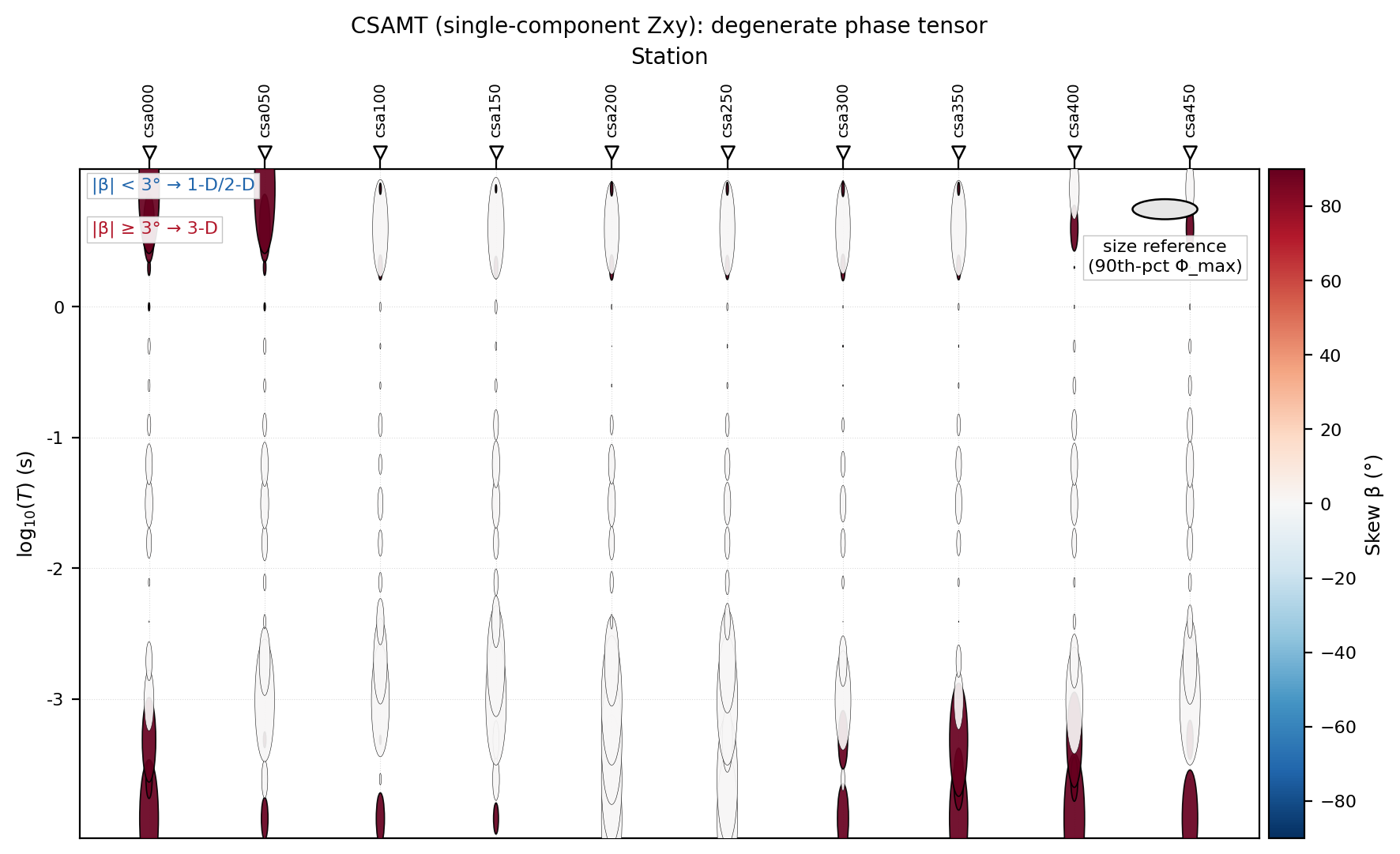
Every ellipse is a zero-width slit, and the fill color alternates between
the two extremes of the skew colorbar with no in-between values – there
is no “moderate skew” here, only the two branches atan2 can return
for a genuinely degenerate matrix. Do not run phase-tensor dimensionality
analysis on single-component CSAMT data and report the result as a real
1-D/2-D/3-D classification; it is a statement about the missing
Zyx component, not about the earth. See also
Source Effects And Near-Field Correction for what this same dataset does look like
under CSAMT-appropriate diagnostics.
11.7.8. Strike As A Director Field#
theta is axial. A director field is often easier to interpret than
a scatter plot because the glyph has no arrow head and therefore
respects the 180-degree ambiguity.
For comparing two strike estimates, use an axial difference rather than
ordinary subtraction:
This keeps differences in the interval \([-90^\circ, 90^\circ]\). Without this adjustment, a harmless jump from \(179^\circ\) to \(1^\circ\) looks like a \(178^\circ\) change instead of a \(2^\circ\) change.
>>> from pycsamt.emtools import plot_strike_director_field
>>> _ = plot_strike_director_field(
...     sites,
...     color_by="skew",
...     length_by="ellipt",
...     skew_max=6.0,
...     streamlines=True,
...     period_subsample=40,
...     recursive=False,
... )
>>> plt.gcf().savefig(
...     "tensor_strike_director_field.png",
...     dpi=200,
...     bbox_inches="tight",
... )
>>> plt.close()
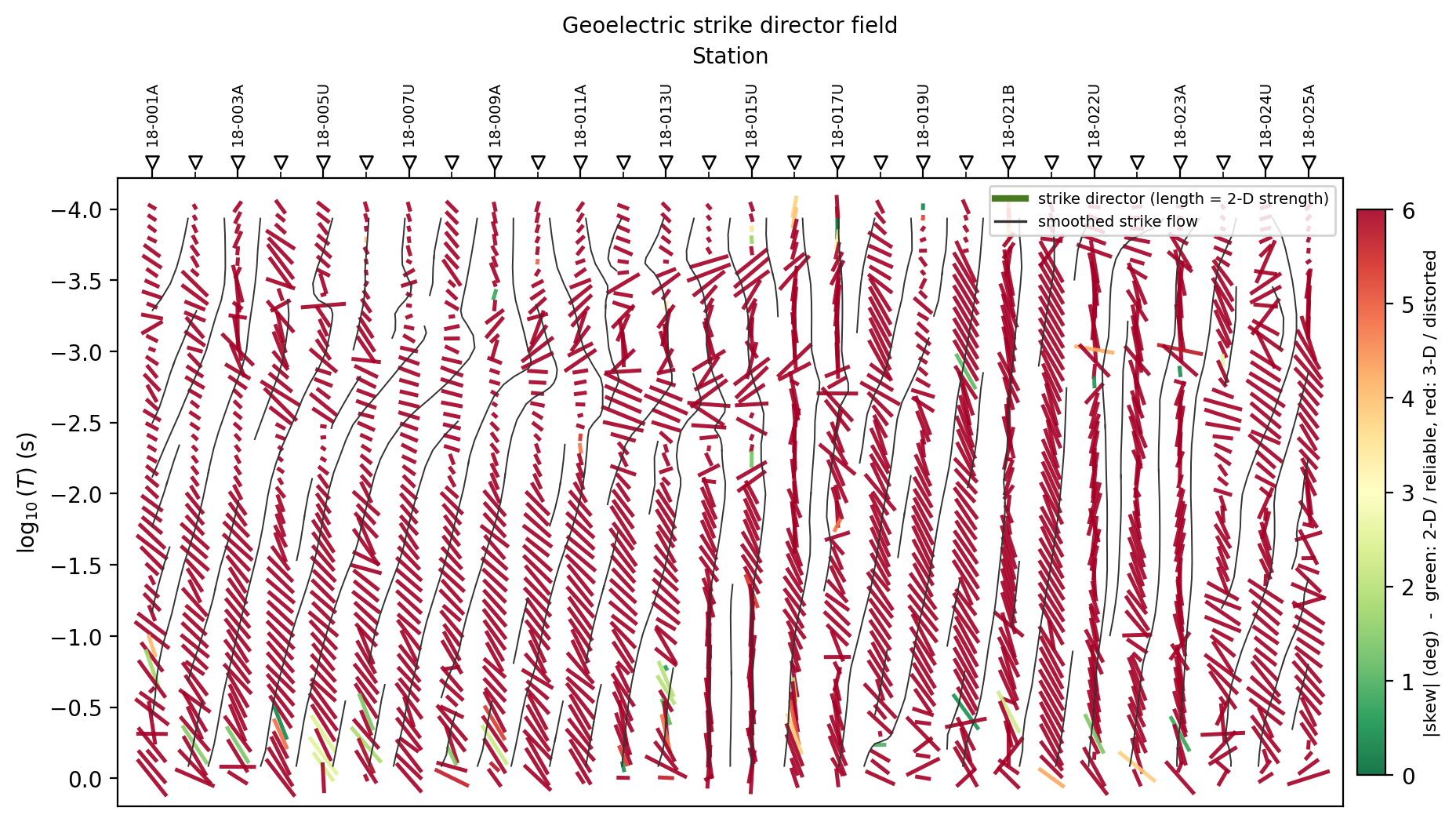
Interpret long, aligned, low-skew directors as a more coherent 2-D strike signal. Short directors mean the phase tensor is close to circular and strike is poorly defined. High-skew directors mean the response is more 3-D or distorted, even if the direction looks visually organized.
11.7.9. Rose And Stability Plots#
Rose plots are useful for summarizing axial direction. Stability plots are useful for seeing whether that summary hides period dependence.
View the executed rose/stability source codeClick to inspect and copy the complete code
 1def make_rose_stability_bundle() -> None:
 2    """Write the three rose/stability figures used by the "Rose And
 3    Stability Plots" section: the overall axial rose, the six-band rose
 4    grid, and the hue/saturation stability stripe.
 5    """
 6    sites = ensure_sites(L18PLT, recursive=True)
 7
 8    plot_phase_tensor_rose(
 9        sites,
10        band=(0.001, 10.0),
11        bins=36,
12        recursive=False,
13    )
14    plt.gcf().savefig(IMAGES / "user-guide-emtools-tensor-09-01.png", dpi=200, bbox_inches="tight")
15    plt.close()
16
17    plot_theta_rose_grid(
18        sites,
19        n_bands=6,
20        bins=24,
21        recursive=False,
22    )
23    plt.gcf().savefig(IMAGES / "user-guide-emtools-tensor-09-02.png", dpi=200, bbox_inches="tight")
24    plt.close()
25
26    plot_theta_stability_stripe(
27        sites,
28        win=5,
29        recursive=False,
30    )
31    plt.gcf().savefig(IMAGES / "user-guide-emtools-tensor-09-03.png", dpi=200, bbox_inches="tight")
32    plt.close()
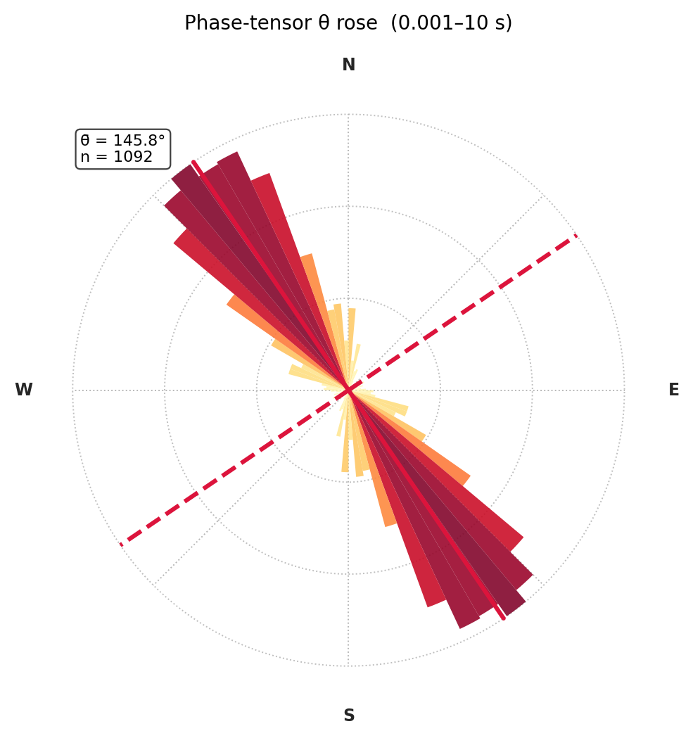

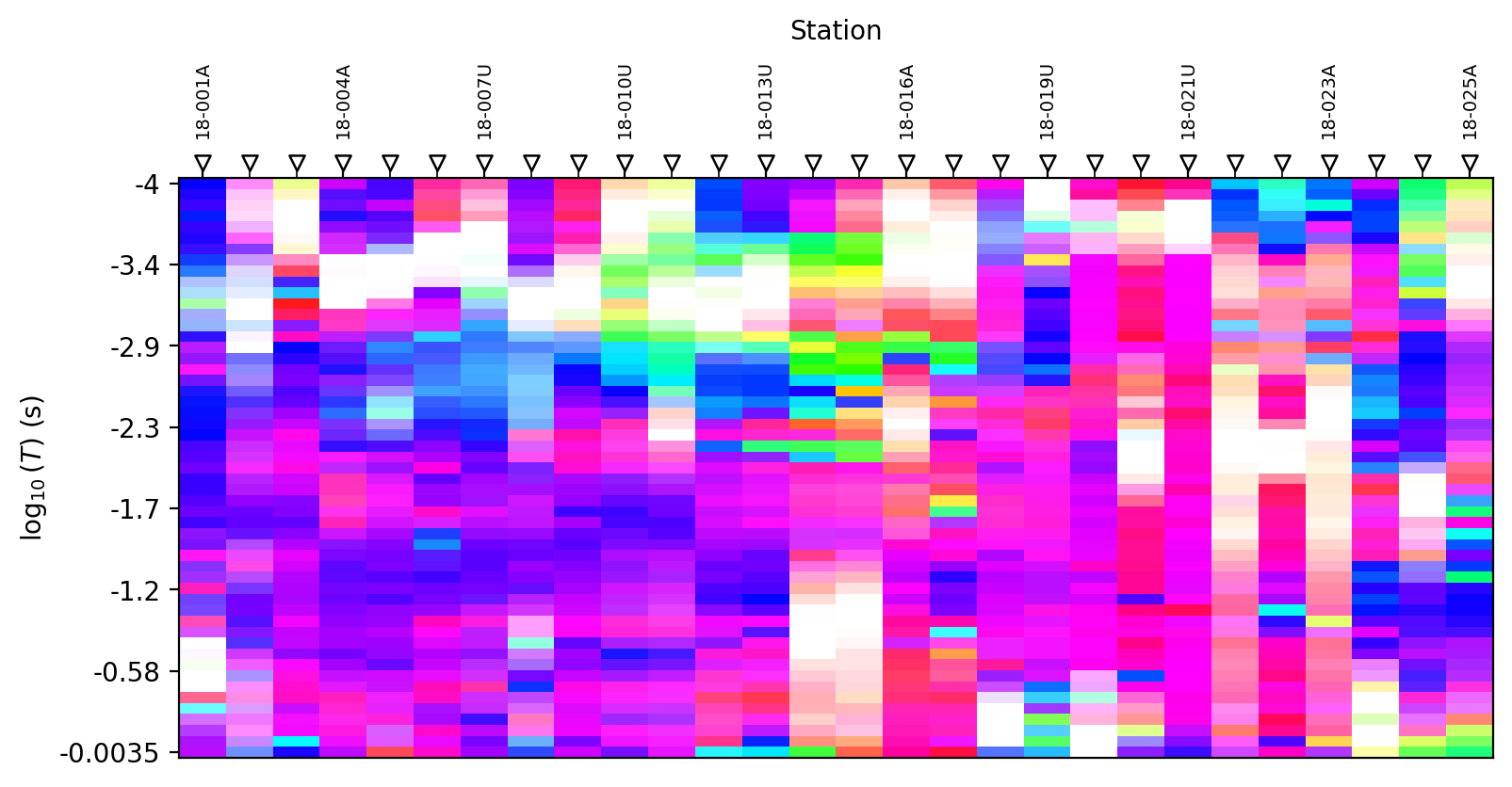
plot_phase_tensor_rose folds all selected theta values into one
axial histogram. plot_theta_rose_grid splits the period range into
equal log-width bands. plot_theta_stability_stripe uses hue for
theta and saturation for local stability.
If the rose grid changes direction from one period band to another, avoid selecting a single strike for the entire data set.
11.7.10. Skew-Ellipticity Density#
plot_skew_ellipt_density shows the joint distribution of
abs(beta) and abs(ellipt). It is a compact way to see whether
the data cluster in a 1-D, 2-D, or 3-D region.
>>> from pycsamt.emtools import plot_skew_ellipt_density
>>> _ = plot_skew_ellipt_density(
...     sites,
...     band=(0.001, 10.0),
...     gridsize=40,
...     recursive=False,
... )
>>> plt.gcf().savefig(
...     "tensor_skew_ellipt_density.png",
...     dpi=200,
...     bbox_inches="tight",
... )
>>> plt.close()
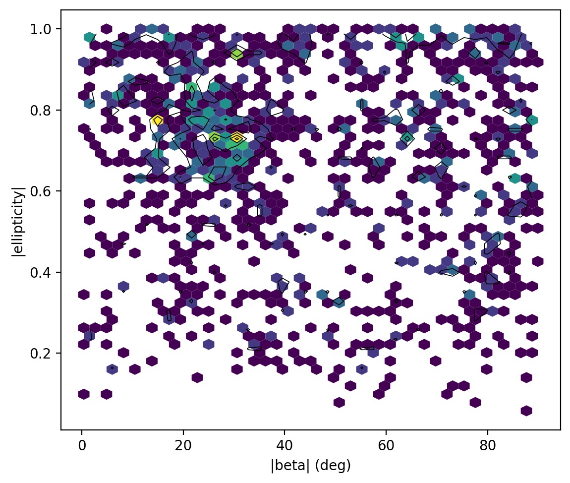
Use this plot with the dimensionality grid. The grid tells you where problem cells occur; the density plot tells you how the full population is distributed.
11.7.11. Summary Figure#
plot_phase_tensor_summary combines the main ellipse pseudosection,
the dimensionality grid, and the skew-ellipticity density into one
figure.
>>> from pycsamt.emtools import plot_phase_tensor_summary
>>> fig = plot_phase_tensor_summary(
...     sites,
...     stations=None,
...     period_range=(0.001, 10.0),
...     c_by="skew",
...     skew_threshold=3.0,
...     ellipt_threshold=0.2,
...     recursive=False,
... )
>>> fig.savefig("tensor_phase_tensor_summary.png", dpi=200, bbox_inches="tight")
>>> plt.close(fig)
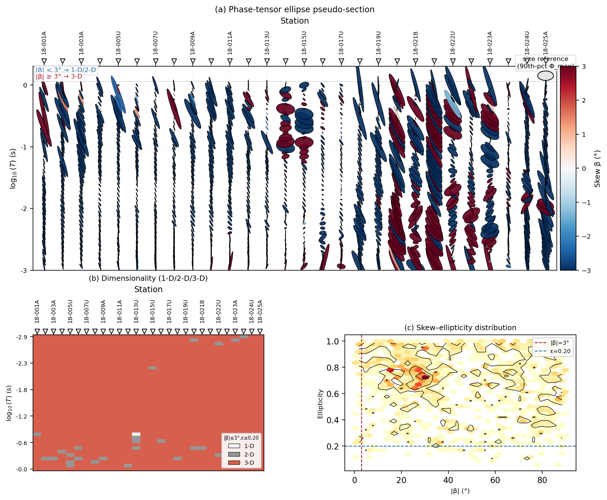
This is a good report figure when the audience needs the whole phase-tensor story in one place: what the ellipses look like, how much of the band is 1-D/2-D/3-D, and where the skew/ellipticity population sits.
11.7.12. Geographic Phase-Tensor Map#
plot_phase_tensor_map draws one phase-tensor ellipse per station at
the period nearest a requested target period. It can also overlay
tipper arrows when vertical magnetic transfer functions are
present.
Each ellipse encodes the phase-tensor shape – its axes are the
principal values \(\Phi_{\max}\) and \(\Phi_{\min}\) and its
long-axis azimuth is the geoelectric strike \(\theta\) – while the
fill colour carries a fourth scalar, by default the skew angle
\(\beta\). A circular, uniformly coloured ellipse indicates a 1-D
response; an elongated ellipse indicates 2-D induction; a strongly
coloured ellipse (large \(|\beta|\)) flags 3-D or galvanically
distorted data. The skew fill uses the diverging pt_skew colormap
(blue for \(\beta<0\), white at \(0\), red for
\(\beta>0\)); pass c_by="|beta|" for the absolute value on the
sequential pt_skew_abs map instead.
Three parameters control how the map reads:
ellipse_scaleA multiplier on the automatic ellipse size.
1.0is the default; values around1.3–1.6make a sparse survey easier to read, while values below1help when ellipses overlap.topographyA convenience elevation background.
Trueinterpolates the station elevations carried in the EDI headers; a path to alon,lat,elev(orstation,elev) CSV supplies an external DEM; a dict is used directly asbg_grid. The interpolation is linear and leaves the area outside the station hull transparent so the background never extrapolates into unsurveyed ground.show_colorbarSet to
Falsewhen tiling several maps that share one figure-level colorbar – this is whatplot_phase_tensor_map_grid()does internally.
>>> from pycsamt.emtools import ensure_sites, plot_phase_tensor_map
>>> bh = ensure_sites("data/MT/broken-hill/edis", recursive=False)
>>> _ = plot_phase_tensor_map(
...     bh,
...     period=0.3,
...     c_by="skew",
...     show_tipper=True,
...     tipper_convention="parkinson",
...     ellipse_scale=1.4,
...     topography=True,
...     station_labels=False,
...     recursive=False,
... )
>>> plt.gcf().savefig("tensor_map_topo.png", dpi=200, bbox_inches="tight")
>>> plt.close()
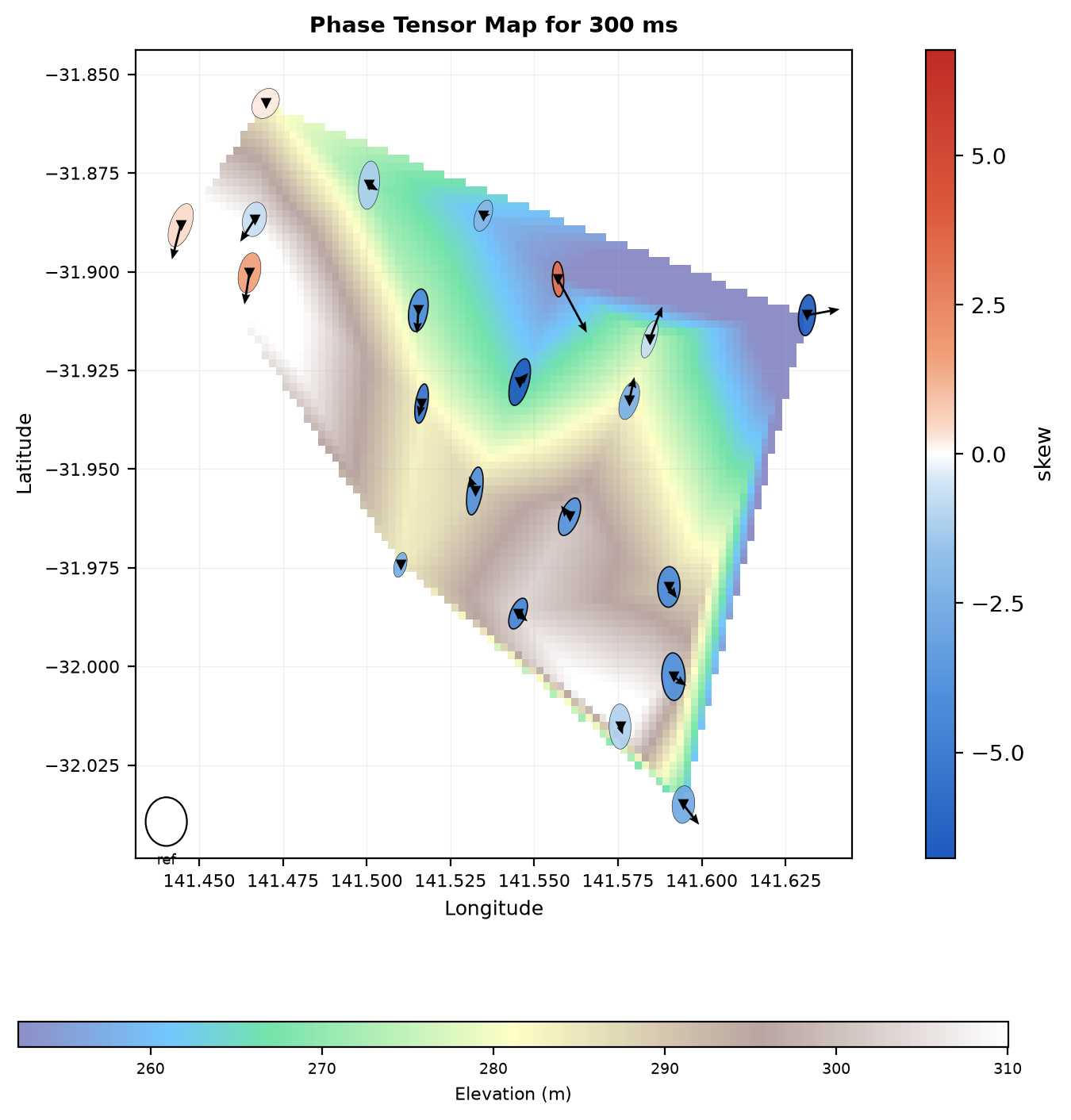
The bundled 21-station Broken Hill MT survey
(data/MT/broken-hill; see its README.md for the data source
and citation) at a 0.3 s target period, on a station-elevation
background.#
At 0.3 s the ellipses are mostly pale blue – small negative skew, consistent with a broadly 2-D to weakly 3-D response – and they are elongated NW–SE, roughly across the regional structural grain. A few stations on the western edge carry longer real induction arrows: in the Parkinson convention the arrow points towards the more conductive side, so those stations sense a lateral conductivity contrast that the interior stations do not. The elevation background is gentle here (about 240–320 m of relief) and is included mainly to show the overlay; on a survey with real topography it helps relate induction arrows to drainage and ridges.
>>> from pycsamt.emtools import plot_phase_tensor_map
>>> _ = plot_phase_tensor_map(
...     sites,
...     period=1.0,
...     c_by="skew",
...     show_tipper=True,
...     tipper_convention="parkinson",
...     station_labels=True,
...     recursive=False,
... )
>>> plt.gcf().savefig("tensor_phase_tensor_map.png", dpi=200, bbox_inches="tight")
>>> plt.close()
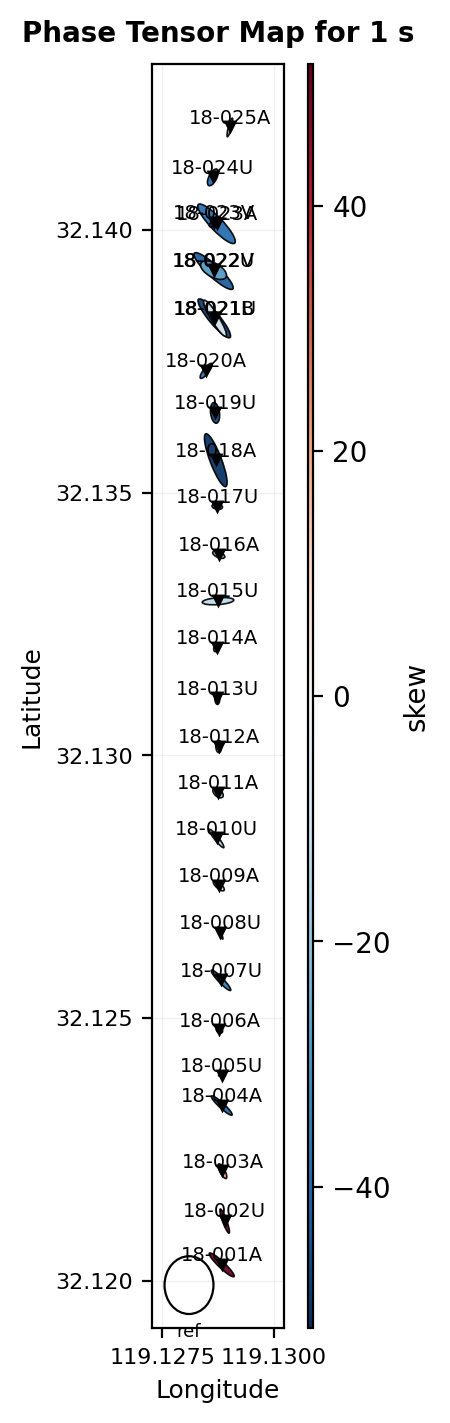
L18PLT is AMT with no vertical-field channel, so show_tipper=True
draws no arrows here; the ellipses are small and pale because the
corrected skew values plotted at period=1.0 second are mostly low.
Use period as a target; each station uses its nearest available
period.
Coordinates come from the EDI header, and getting them right matters for
every figure in this section. build_phase_tensor_table and the
pseudosection functions above never needed station positions, but the
map does – and coordinate parsing has its own failure modes worth
knowing about.
11.7.13. Real Tipper On A Real Map#
data/MT/kap03lmt_edis is a real 26-station SAMTEX MT line that,
unlike L18PLT, does carry genuine vertical-field data, which makes it
the right dataset to see real tipper arrows on a real phase-tensor map.
>>> kap = ensure_sites("data/MT/kap03lmt_edis", recursive=True, verbose=0)
>>> n_valid = sum(
...     1 for s in kap
...     if s.coords and np.isfinite(s.coords[0]) and np.isfinite(s.coords[1])
... )
>>> print("kap03 stations with usable coordinates:", n_valid, "/", len(kap))
kap03 stations with usable coordinates: 26 / 26
>>> _ = plot_phase_tensor_map(
...     kap,
...     period=10.0,
...     c_by="skew",
...     show_tipper=True,
...     tipper_convention="parkinson",
...     station_labels=False,
...     recursive=False,
... )
>>> plt.gcf().savefig("tensor_phase_tensor_map_kap03.png", dpi=200, bbox_inches="tight")
>>> plt.close()
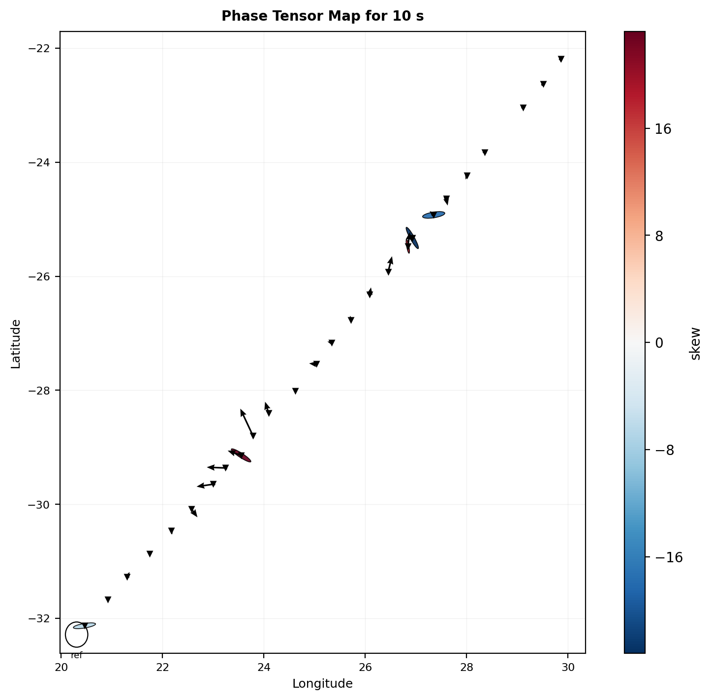
All 26 stations get a real position, and several carry visible induction
arrows and ellipses along the profile. That “26 / 26” is worth pausing
on: these EDI files are older BIRRP-processed output that never fill in
the ordinary LAT=/LONG= keys inside >HEAD. What they do
carry is REFLAT/REFLONG inside >=DEFINEMEAS – a real,
if less common, coordinate convention. Site.coords now falls back to
that block automatically whenever the header alone cannot supply a
field, which is what makes this map possible at all; without that
fallback every one of these 26 stations would report (nan, nan) and
every coordinate-based tool on this page would silently draw nothing for
this survey.
11.7.14. When Header Coordinates Are Noisy#
Coordinates existing is not the same as coordinates being trustworthy.
data/CSAMT does carry header positions – via the same
REFLAT/REFLONG fallback – but they come from field GPS fixes
along a short, 450 m line, and GPS jitter at that scale is a real,
common problem.
>>> csamt2 = ensure_sites("data/CSAMT", recursive=False, verbose=0)
>>> n_valid_csamt = sum(
...     1 for s in csamt2
...     if s.coords and np.isfinite(s.coords[0]) and np.isfinite(s.coords[1])
... )
>>> print("CSAMT stations with usable header coordinates:", n_valid_csamt, "/", len(csamt2))
CSAMT stations with usable header coordinates: 10 / 10
>>> _ = plot_phase_tensor_map(
...     csamt2,
...     period=0.01,
...     show_tipper=False,
...     station_labels=True,
...     recursive=False,
... )
>>> plt.gcf().savefig("tensor_phase_tensor_map_csamt_header.png", dpi=200, bbox_inches="tight")
>>> plt.close()
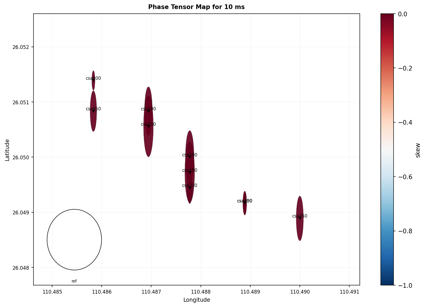
The header positions are real GPS fixes, but they do not trace a clean
straight line: compare csa300, which sits offset to the northwest of
the csa250-csa200 trend instead of continuing it. The station
names themselves encode the true, intended design – a straight transect
at 50 m spacing, exactly what a CSAMT along-line survey is built to
be. When you know the true local geometry better than a handful of GPS
fixes do, override it explicitly with coords:
>>> coords = {
...     "csa000": (0.0, 0.0),
...     "csa050": (0.0, 50.0),
...     "csa100": (0.0, 100.0),
...     "csa150": (0.0, 150.0),
...     "csa200": (0.0, 200.0),
...     "csa250": (0.0, 250.0),
...     "csa300": (0.0, 300.0),
...     "csa350": (0.0, 350.0),
...     "csa400": (0.0, 400.0),
...     "csa450": (0.0, 450.0),
... }
>>> _ = plot_phase_tensor_map(
...     csamt2,
...     period=0.01,
...     coords=coords,
...     show_tipper=False,
...     station_labels=True,
...     recursive=False,
... )
>>> plt.gcf().savefig(
...     "tensor_phase_tensor_map_custom_coords.png",
...     dpi=200,
...     bbox_inches="tight",
... )
>>> plt.close()
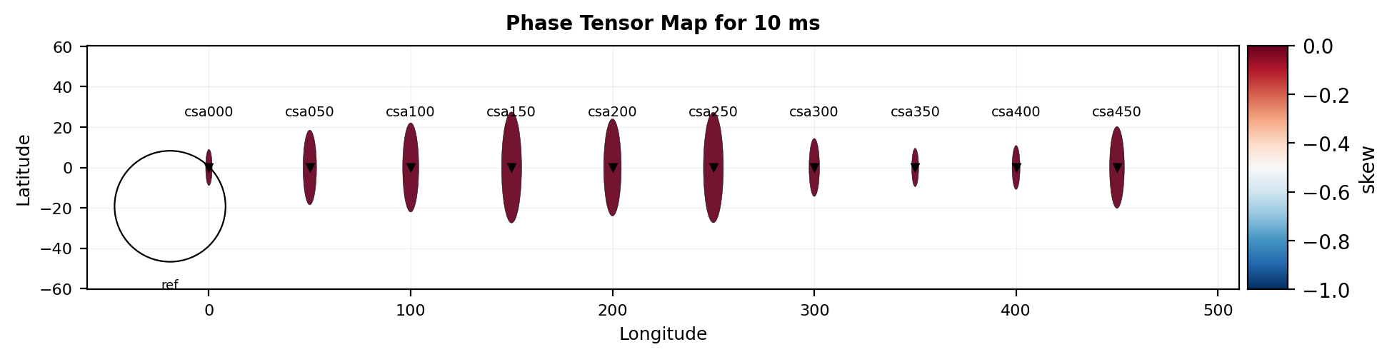
The coordinate tuple is (lat, lon) for header-derived positions, but
coords accepts any consistent 2-D frame – here a local along-line
grid in meters, which is both more physically meaningful for a CSAMT
transect and immune to header GPS noise. Reach for coords whenever
the header disagrees with better-known survey geometry, not only when a
map silently comes up empty.
11.7.15. Multi-Frequency Phase-Tensor Maps#
A phase-tensor map at a single period answers “what does the response
look like at this depth of investigation?”. The dimensionality and
geoelectric strike almost always change with period, so the more useful
figure is a small grid of maps at several frequencies, read together.
plot_phase_tensor_map_grid tiles plot_phase_tensor_map() across
a list of frequencies (or periods) with one shared colour scale, one
shared ellipse-size reference, and a single figure-level colorbar, so
the panels are directly comparable.
>>> from pycsamt.emtools import plot_phase_tensor_map_grid
>>> fig = plot_phase_tensor_map_grid(
...     bh,
...     frequencies=[30.0, 3.0, 0.3, 0.03],
...     c_by="skew",
...     tipper_convention="parkinson",
...     ellipse_scale=1.3,
...     station_labels="none",
...     ref_ellipse="none",
...     suptitle="Broken Hill -- phase tensor (skew) + Parkinson arrows",
...     recursive=False,
... )
>>> fig.savefig("tensor_map_grid.png", dpi=200, bbox_inches="tight")
>>> plt.close(fig)
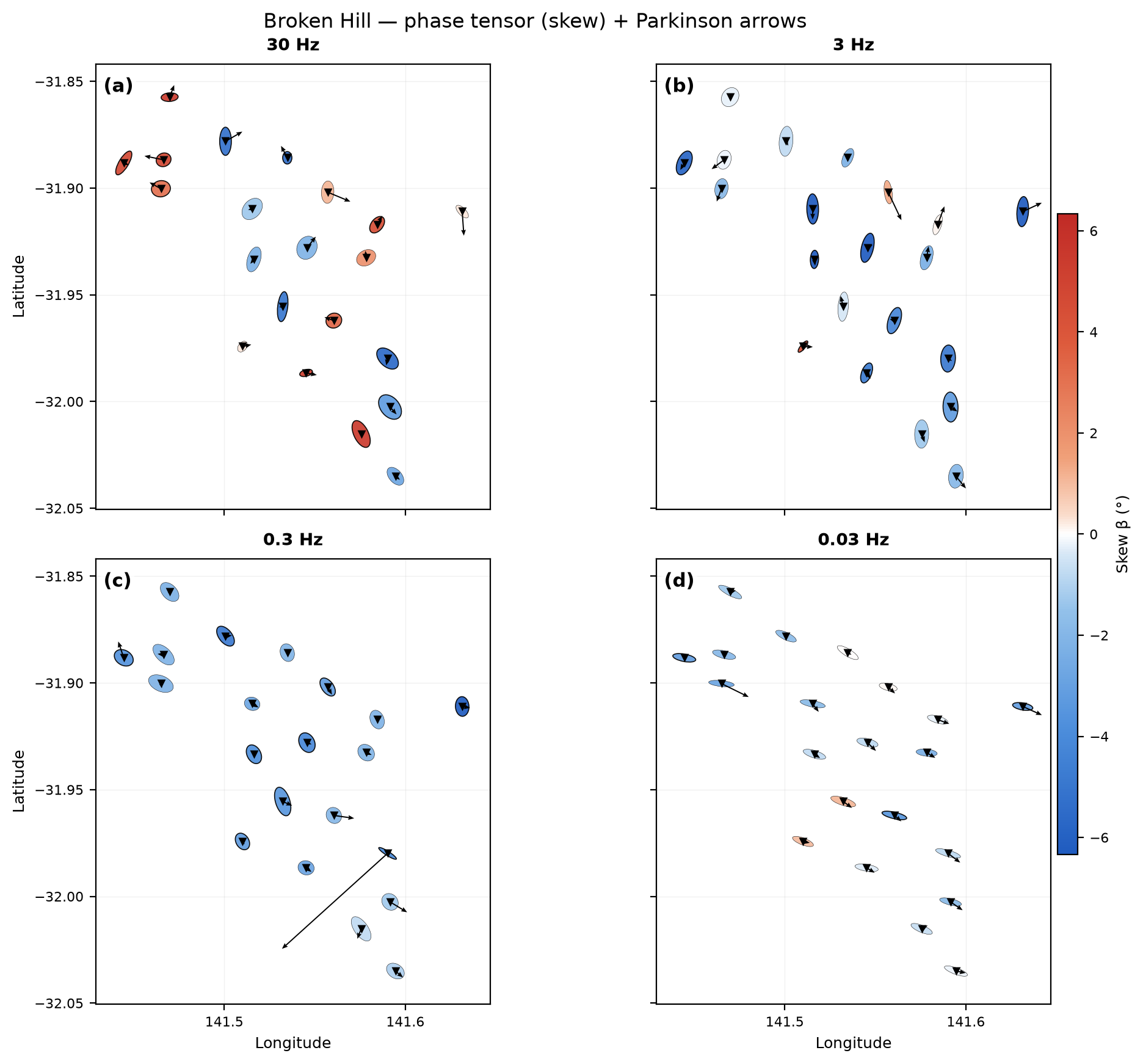
The same Broken Hill survey at 30, 3, 0.3 and 0.03 Hz. Panel labels, per-panel frequency titles, the shared skew colorbar, and the tightened grid layout are all produced automatically.#
Read across the panels rather than down them. At 30 Hz (shallowest) the skew is a mix of blue and red – several stations exceed \(|\beta|\approx3^\circ\), the usual threshold for calling a response 3-D – and the ellipses are short and variably oriented. By 0.03 Hz (deepest) almost every ellipse is a similar pale blue and the long axes have settled into a consistent NW–SE orientation. The physical reading is a shallow section broken up by near-surface 3-D structure, over a deeper section that behaves as a coherent 2-D layer with a stable regional strike – exactly the situation where a single-period map would mislead.
frequencies accepts any number of entries; the layout adapts (one
column for one panel, 2 x 2 for four, three per row beyond that) and
n_cols overrides it. periods in seconds is the alternative to
frequencies in hertz. Two further controls matter for comparability
across a grid:
share_scaleOn by default. It fixes a single geographic ellipse scale for every panel, but lets each panel normalise ellipse sizes to its own phase distribution – otherwise the small, high-frequency phase tensors would collapse to points beside the large low-frequency ones. Pass an explicit
s1_refwhen you specifically want ellipse area to be comparable across frequency.abs_skewA shorthand for
c_by="|beta|". The absolute skew removes the sign and uses the sequentialpt_skew_abscolormap, which makes a “where is the data 3-D?” map easier to scan than the signed version.
>>> fig = plot_phase_tensor_map_grid(
...     bh,
...     frequencies=[30.0, 0.3],
...     abs_skew=True,
...     tipper_convention="parkinson",
...     station_labels="none",
...     ref_ellipse="none",
...     suptitle="Broken Hill -- |skew| (2-D vs 3-D character)",
...     recursive=False,
... )
>>> fig.savefig("tensor_map_grid_abs.png", dpi=200, bbox_inches="tight")
>>> plt.close(fig)
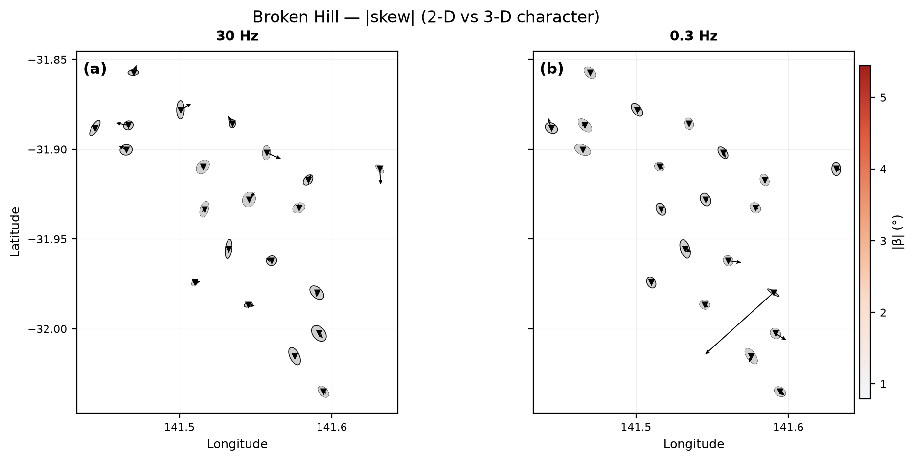
Absolute skew at 30 Hz and 0.3 Hz. The darker cells at 30 Hz mark the stations where a 2-D inversion assumption is least safe; by 0.3 Hz almost all of them have faded towards white.#
Every keyword that plot_phase_tensor_map() accepts – bg_grid,
topography, tipper_component, tipper_scale, the ellipse-style
options – is forwarded to each panel, so the grid is a drop-in
replacement whenever you find yourself calling the single-period map more
than once for the same survey.
11.7.16. Per-Station Ellipse Strips#
plot_phase_tensor_strip draws one station as an ellipse sequence
through period. plot_phase_tensor_strip_grid tiles several such
strips, optionally grouped by profile.
>>> from pycsamt.emtools import (
...     plot_phase_tensor_strip,
...     plot_phase_tensor_strip_grid,
... )
>>> _ = plot_phase_tensor_strip(
...     sites,
...     station="18-016A",
...     period_range=(0.001, 10.0),
...     c_by="skew",
...     recursive=False,
... )
>>> plt.gcf().savefig("tensor_phase_tensor_strip.png", dpi=200, bbox_inches="tight")
>>> plt.close()
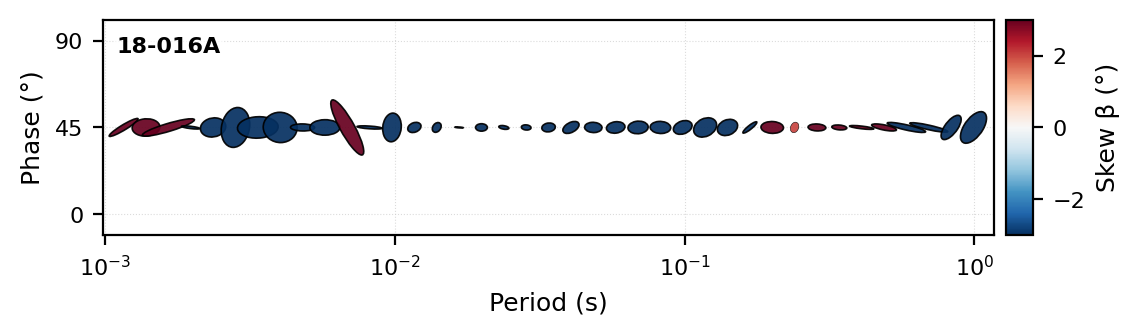
Station 18-016A was already flagged in the numeric summary as one of
the better-behaved stations (median absolute skew 12.1 degrees), and
the strip confirms it: colors stay within about ±3 degrees of white
across almost the whole period range.
>>> groups = {
...     "L18PLT": ["18-001A", "18-002U", "18-003A", "18-004A"],
... }
>>> _ = plot_phase_tensor_strip_grid(
...     sites,
...     groups,
...     period_range=(0.001, 10.0),
...     c_by="skew",
...     recursive=False,
... )
>>> plt.gcf().savefig(
...     "tensor_phase_tensor_strip_grid.png",
...     dpi=200,
...     bbox_inches="tight",
... )
>>> plt.close()
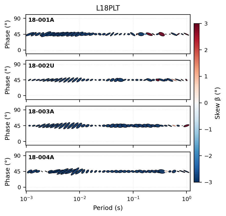
All four stations in this group show the same broad pattern: cooler (blue, negative-skew) ellipses at short period giving way to a run of saturated dark-red cells in the middle of the band. A shared pattern across neighboring stations is more likely to be real structure than a single-station artifact. Use strips when a single station deserves close inspection. Use the grid when comparing stations or profile groups without the compression of a full pseudosection.
11.7.17. Standalone Legend#
phase_tensor_legend draws a reference ellipse that can be composed
into custom figures.
>>> from pycsamt.emtools import phase_tensor_legend
>>> _ = phase_tensor_legend(size=1.0)
>>> plt.gcf().savefig("tensor_phase_tensor_legend.png", dpi=200, bbox_inches="tight")
>>> plt.close()
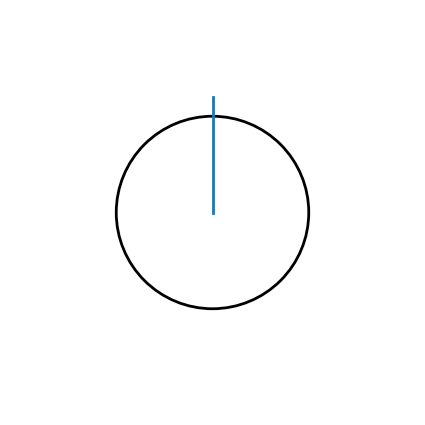
It is not a diagnostic by itself; it is a small plotting component for figures where the phase-tensor ellipse convention needs to be explained.
11.7.18. Impedance-Tensor Editing#
Tensor editing functions change Z. They should be treated as
processing operations, not as harmless plots. Keep inplace=False
unless you deliberately want to mutate the object in memory.
The rotation convention used by the tensor tools is a strike
rotation-style congruence rotation of the horizontal coordinate frame:
A fixed-angle rotation applies the same \(\alpha\) everywhere.
rotate_by_map lets \(\alpha=\alpha_s\) vary by station, and
rotate_z_to_strike estimates an angle before applying the same
operation. Because rotation mixes all four tensor components, always
compare phase-tensor and impedance diagnostics before and after.
Function |
What it does |
Typical use |
|---|---|---|
|
Rotates all station impedance tensors by one fixed angle. |
Apply a known regional strike or sensor-frame correction. |
|
Rotates each station by a value from a station-angle dictionary. |
Apply station-specific rotations from an external interpretation. |
|
Estimates a tensor strike for each station and rotates by it. |
Exploratory tensor-level strike rotation. |
|
Enforces off-diagonal antisymmetry. |
Prepare data for methods that assume |
|
Corrects electric and magnetic sensor orientations. |
Fix known sensor azimuth errors. |
|
Sets outlying |
Remove isolated spikes before plotting or inversion. |
|
Balances off-diagonal magnitudes. |
Exploratory symmetry conditioning. |
|
Replaces each 2-by-2 impedance tensor by its matrix inverse. |
Advanced workflows that explicitly need admittance-like tensors. |
11.7.19. Fixed-Angle Rotation#
Use rotate when every station should receive the same angle.
>>> from pycsamt.emtools import rotate
>>> rotated_30 = rotate(
...     sites,
...     30.0,
...     inplace=False,
...     recursive=False,
... )
Use this only when the angle is justified by strike analysis, field geometry, or a documented processing convention.
11.7.20. Station-Specific Rotation#
Use rotate_by_map when each station needs its own angle.
>>> from pycsamt.emtools import rotate_by_map
>>> angle_by_station = {
...     "18-001A": 25.0,
...     "18-002A": 27.5,
...     "18-003A": 24.0,
... }
>>> rotated_stationwise = rotate_by_map(
...     sites,
...     angle_by_station,
...     inplace=False,
...     recursive=False,
... )
Stations missing from the dictionary receive a 0 degree rotation.
For production work, check that every intended station is present in the
map before applying it.
11.7.21. Tensor Rotation To Strike#
The tensor module’s rotation-to-strike function is exported as
rotate_z_to_strike at the pycsamt.emtools level. This avoids a
name collision with the strike module’s rotate_to_strike.
>>> from pycsamt.emtools import rotate_z_to_strike
>>> rotated_to_tensor_strike = rotate_z_to_strike(
...     sites,
...     method="swift",
...     inplace=False,
...     recursive=False,
... )
Use this as a tensor editing step, not as the main strike-analysis interface. For detailed strike estimation, use the dedicated Geoelectric Strike workflow and its station-level tables.
11.7.22. Antisymmetrize And Balance#
antisymmetrize enforces off-diagonal antisymmetry. balance_offdiag
balances |Zxy| and |Zyx| while preserving phase.
For an off-diagonal pair \(Z_{xy}\) and \(Z_{yx}\),
antisymmetrization replaces the pair by a common antisymmetric target,
schematically
where \(A\) is chosen by the backend utility according to how.
With how="rms", the target amplitude is tied to the root-mean-square
scale of the two original off-diagonal terms.
balance_offdiag(mode="avgabs") keeps each component phase but gives
both off-diagonal terms the same magnitude
This is gentler than antisymmetrization because it does not force a 180-degree phase relationship.
>>> from pycsamt.emtools import antisymmetrize, balance_offdiag
>>> antisymmetric = antisymmetrize(
...     sites,
...     how="rms",
...     inplace=False,
...     recursive=False,
... )
>>> balanced = balance_offdiag(
...     sites,
...     mode="avgabs",
...     inplace=False,
...     recursive=False,
... )
These operations can be useful for controlled experiments or for
preparing data for algorithms with strong 2-D assumptions. They can
also hide real 3-D information if applied blindly. Always keep an
uncorrected copy. antisymmetrize is not a fix for the CSAMT
single-component case shown above: forcing Zyx = -Zxy when Zyx
was never measured manufactures a value rather than recovering one, and
the resulting phase tensor would look plausible without being real.
11.7.23. Sensor Orientation#
Use orient_from_sensors when field notes show that the electric and
magnetic sensors were not aligned with the assumed axes.
>>> from pycsamt.emtools import orient_from_sensors
>>> oriented = orient_from_sensors(
...     sites,
...     ex=5.0,
...     ey=95.0,
...     bx=5.0,
...     by=95.0,
...     degrees=True,
...     inplace=False,
...     recursive=False,
... )
Angles are degrees by default. Pass degrees=False only when your
inputs are radians. This operation is meaningful only when the sensor
orientation metadata or field notes are trustworthy.
11.7.24. Sigma Clip Outliers#
sigma_clip_z flags outlying entries in the complex impedance tensor
and sets them to NaN.
The clipping mask is applied component-wise to complex entries. In plain statistical terms, a value is rejected when its standardized departure exceeds the requested threshold:
After clipping, rerun coverage and QC checks. A small number of clipped entries may remove isolated spikes; a large number means the survey or threshold needs review.
>>> from pycsamt.emtools import sigma_clip_z
>>> clipped = sigma_clip_z(
...     sites,
...     sigma=3.0,
...     inplace=False,
...     recursive=False,
... )
11.7.25. Invert Tensor#
invert applies the 2-by-2 matrix inverse frequency by frequency.
For each frequency,
>>> from pycsamt.emtools import invert
>>> admittance_like = invert(
...     sites,
...     inplace=False,
...     recursive=False,
... )
This is an advanced operation. Do not use it as a generic noise correction. It changes the physical quantity represented by the tensor.
11.7.26. Audit Edits With Phase-Tensor Tables#
A safe editing workflow compares before and after diagnostics.
>>> before = build_phase_tensor_table(sites, recursive=False)
>>> rotated = rotate(
...     sites,
...     30.0,
...     inplace=False,
...     recursive=False,
... )
>>> after = build_phase_tensor_table(rotated, recursive=False)
>>> audit = before[["station", "period", "theta", "skew", "ellipt"]].merge(
...     after[["station", "period", "theta", "skew", "ellipt"]],
...     on=["station", "period"],
...     suffixes=("_before", "_after"),
... )
>>> audit["theta_change"] = (
...     (audit["theta_after"] - audit["theta_before"] + 90.0) % 180.0
... ) - 90.0
>>> print(audit[["station", "period", "theta_change", "skew_before", "skew_after"]])
      station    period  theta_change  skew_before  skew_after
0     18-001A  0.000096         -30.0     2.611588    2.611588
1     18-001A  0.000115         -30.0     1.964321    1.964321
2     18-001A  0.000137         -30.0     1.804266    1.804266
3     18-001A  0.000164         -30.0     1.068855    1.068855
4     18-001A  0.000196         -30.0    -6.949269   -6.949269
...       ...       ...           ...          ...         ...
1479  18-025A  0.487329         -30.0   -20.351504  -20.351504
1480  18-025A  0.582072         -30.0   -46.015322  -46.015322
1481  18-025A  0.695410         -30.0   -73.461943  -73.461943
1482  18-025A  0.830565         -30.0   -87.940352  -87.940352
1483  18-025A  0.992063         -30.0    86.240927   86.240927

[1484 rows x 5 columns]
>>> fig = plot_phase_tensor_summary(
...     rotated,
...     period_range=(0.001, 10.0),
...     recursive=False,
... )
>>> fig.savefig("tensor_audit_summary.png", dpi=200, bbox_inches="tight")
>>> plt.close(fig)
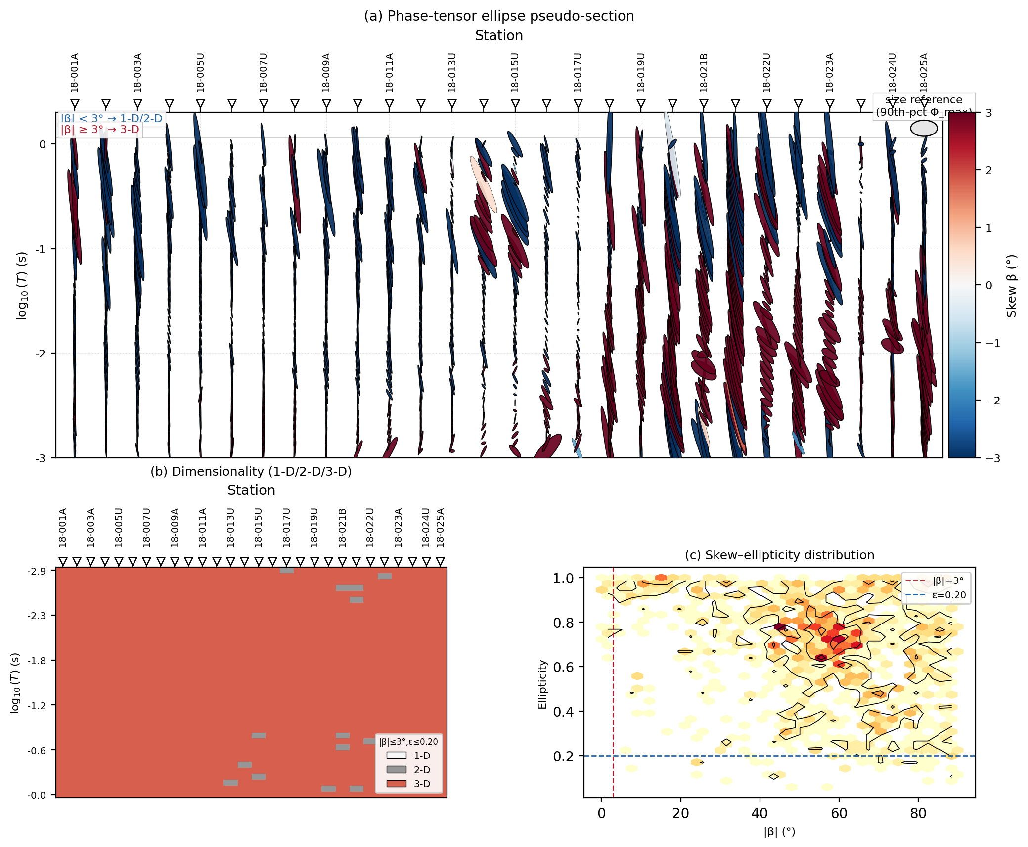
theta_change is exactly -30 degrees for every single row – the
axial difference formula correctly tracks a uniform \(30^\circ\)
rotation across the whole survey. skew_before and skew_after are
identical to six decimal places for every row too, and that is not a
coincidence: \(\beta\) was defined specifically to be invariant under
this rotation, and a real 1484-row audit on field data confirms the
theory holds in practice. If you ever rotate a survey and see skew
change, treat that as a signal something in the pipeline – not the
physics – is wrong.
11.7.27. Recommended Interpretation Workflow#
For a survey report, keep the phase-tensor interpretation explicit. The script below builds the table, the core ellipse pseudosection, a period-band rose grid, the skew-ellipticity density, and a full summary figure, all from the same period range and thresholds.
View the executed recommended-workflow source codeClick to inspect and copy the complete code
 1def run_recommended_workflow() -> None:
 2    """Build the core pseudosection, rose grid, density plot, and summary
 3    figure used by the "Recommended Interpretation Workflow" section,
 4    all with the same period band and thresholds.
 5    """
 6    sites = ensure_sites(L18PLT, recursive=True)
 7
 8    period_range = (0.001, 10.0)
 9    skew_threshold = 3.0
10    ellipt_threshold = 0.2
11
12    plot_phase_tensor_psection(
13        sites,
14        period_range=period_range,
15        c_by="skew",
16        skew_threshold=skew_threshold,
17        mark_3d=True,
18        recursive=False,
19    )
20    plt.gcf().savefig(IMAGES / "user-guide-emtools-tensor-24-01.png", dpi=200, bbox_inches="tight")
21    plt.close()
22
23    plot_theta_rose_grid(
24        sites,
25        n_bands=6,
26        recursive=False,
27    )
28    plt.gcf().savefig(IMAGES / "user-guide-emtools-tensor-24-02.png", dpi=200, bbox_inches="tight")
29    plt.close()
30
31    plot_skew_ellipt_density(
32        sites,
33        band=period_range,
34        recursive=False,
35    )
36    plt.gcf().savefig(IMAGES / "user-guide-emtools-tensor-24-03.png", dpi=200, bbox_inches="tight")
37    plt.close()
38
39    fig = plot_phase_tensor_summary(
40        sites,
41        period_range=period_range,
42        skew_threshold=skew_threshold,
43        ellipt_threshold=ellipt_threshold,
44        recursive=False,
45    )
46    fig.savefig(IMAGES / "user-guide-emtools-tensor-24-04.png", dpi=200, bbox_inches="tight")
47    plt.close(fig)
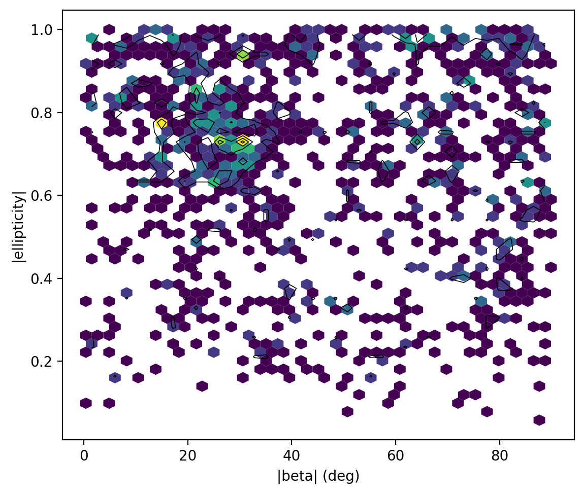
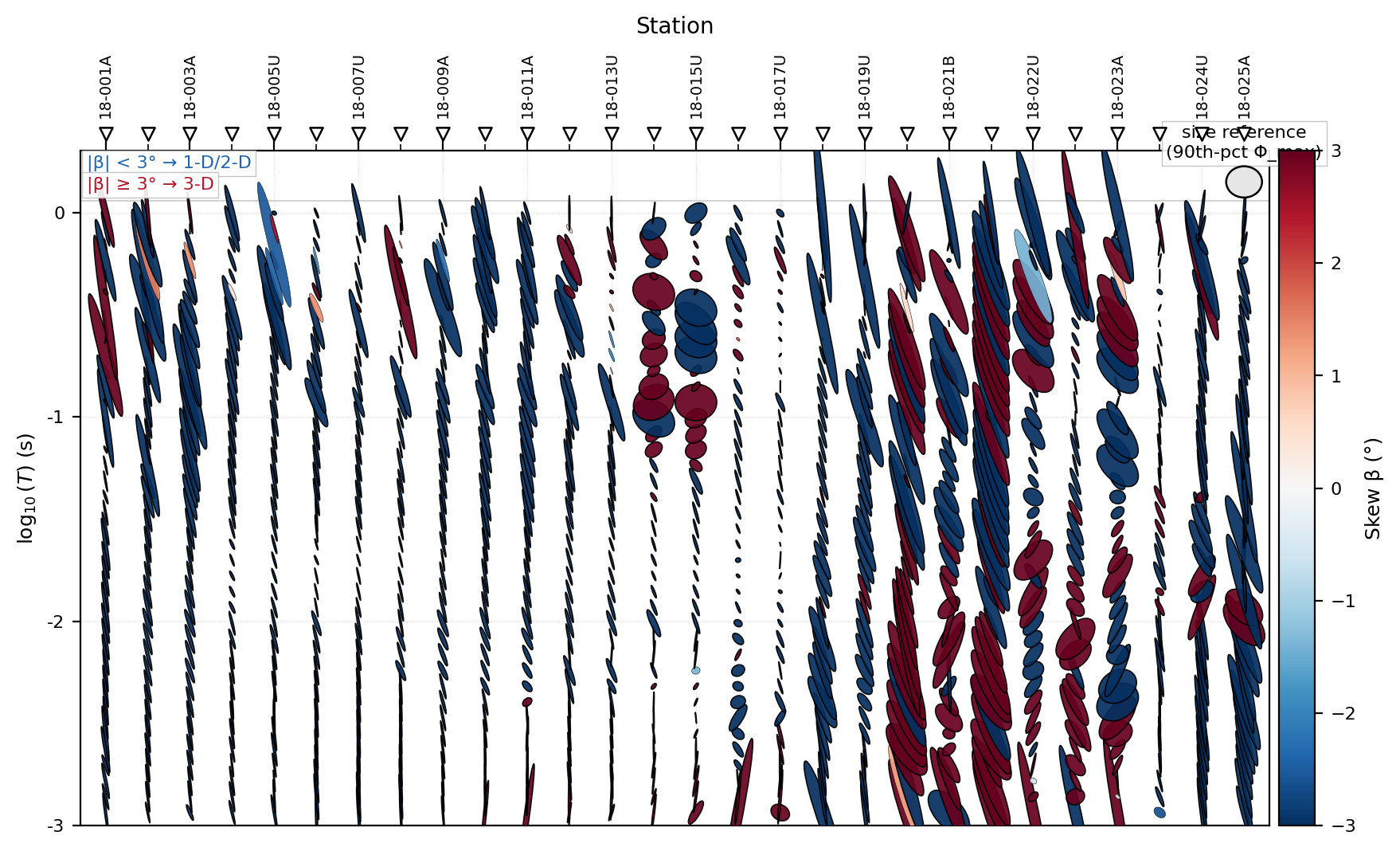

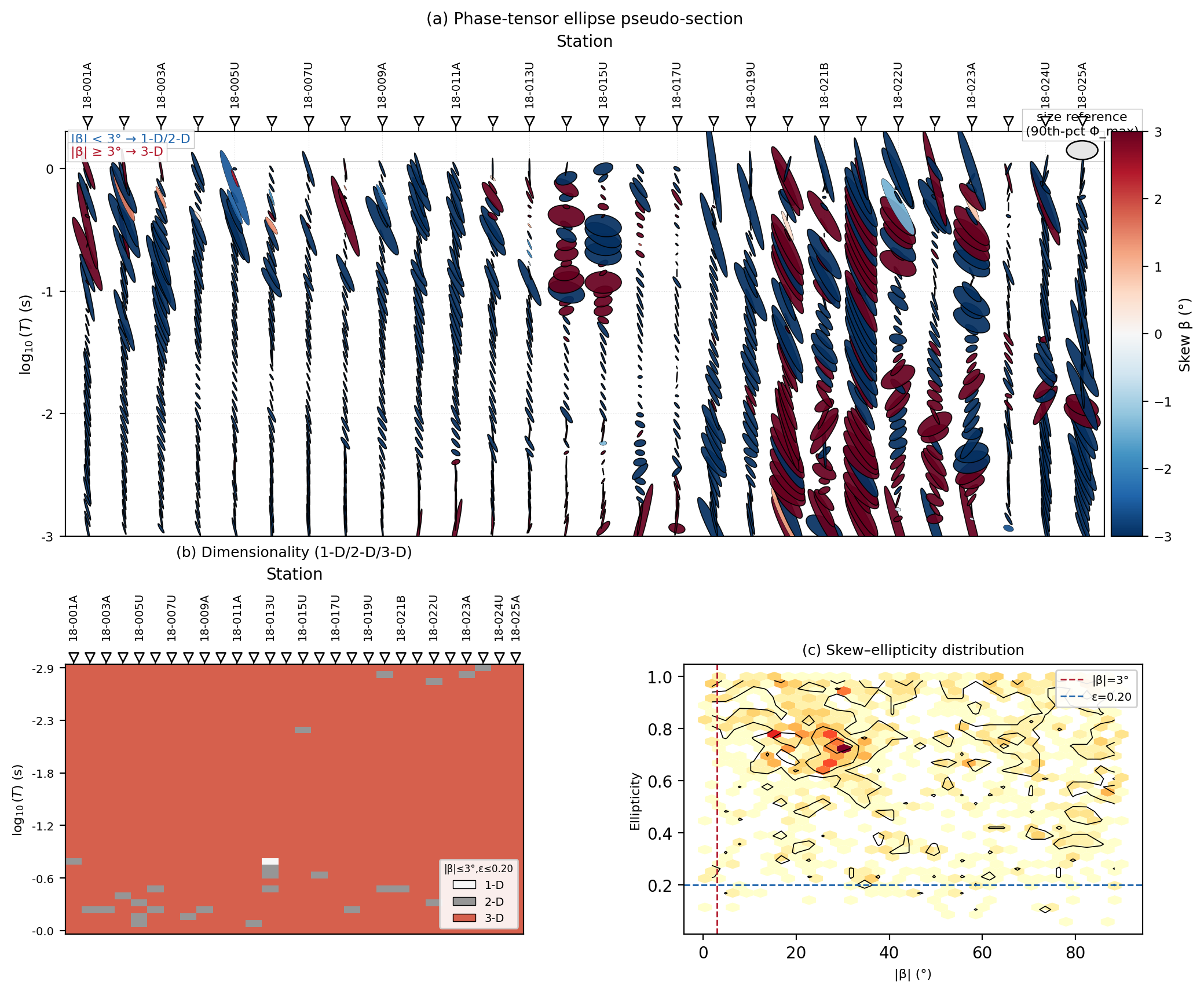
This workflow plots the core ellipse section, checks strike by band,
checks skew/ellipticity distribution, and creates a summary figure with
the same thresholds used everywhere else on this page (1092 rows in
the (0.001, 10.0) second band, median |skew| of 16.9 degrees
– matching the “Filter By Period” section exactly, since it is the same
survey and the same band).
11.7.28. Common Pitfalls#
Do not treat theta as an ordinary linear angle. It is axial. Use an
axial difference formula when comparing directions.
Do not rotate data only because a strike value exists. High skew,
unstable theta, or strong period dependence can make the rotation
misleading.
Do not hide 3-D behavior by editing Z too early. Plot the raw phase
tensor before applying antisymmetrization, balancing, clipping, or
rotation.
Do not run phase-tensor dimensionality analysis on single-component data.
A missing Zyx (or Zxy) produces a mathematically degenerate,
exactly-singular phase tensor – ellipt pinned at 1, s2
pinned at 0 – that looks like a plot, not like an error message, but
carries no real dimensionality information.
Do not assume a missing map means missing tensor data, and do not assume
a rendered map means trustworthy coordinates. Both LAT=/LONG=
header keys and REFLAT/REFLONG in >=DEFINEMEAS are checked
automatically, but header GPS fixes can still be noisy; compare against
known survey geometry and pass an explicit coords mapping when the
header disagrees with it.
Do not mix the two rotation-to-strike functions. Use
rotate_z_to_strike for the tensor editing helper exported from
pycsamt.emtools. Use the dedicated strike page for the strike module
workflow.
11.7.29. Worked Example#
The gallery example computes the phase-tensor table, builds the main pseudosections and rose diagrams, demonstrates the map and strip views, and audits impedance-tensor editing operations on real data.
Open the rendered gallery page here: Phase-tensor analysis and tensor editing (pycsamt.emtools.tensor).