
1.10. View Controls#
pycsamt.api.control is the smallest of the display-configuration
families, and the only one with no named presets: it holds three leaf
controls – phase wrapping, apparent resistivity scale, and the
frequency/period axis convention – that most pycsamt.emtools
plotting functions read by default through
PYCSAMT_CONTROL. Multi-Station Diagnostic Panels
already shows it wired into a real function call end to end; this page
covers what each control actually computes.
>>> from pathlib import Path
>>> from pycsamt.emtools import ensure_sites
>>> from pycsamt.api.control import PYCSAMT_CONTROL

>>> edi_dir = Path("data/AMT/WILLY_DATA/L18PLT")
>>> sites = ensure_sites(
...     edi_dir,
...     recursive=True,
...     on_dup="replace",
...     strict=False,
...     verbose=0,
... )
>>> st = sites["18-001A"]
>>> freq = st.freq
>>> rho_xy = st.rho[:, 0, 1]

>>> print(PYCSAMT_CONTROL)
PyCSAMTControl
  phase.range = (-180.0, 180.0)
  phase.unit  = 'degree'
  phase.wrap  = True
  rho.view    = 'log10'
  x.view      = 'log10_period'
1.10.1. Phase View Control#
PhaseViewControl wraps phase values into a
configurable interval – (-180, 180) by default – using
wrap_phase(), a plain modulo:
Values already inside the interval pass through unchanged; values outside it fold back in, which is what makes it useful for XY/YX components whose raw phase can sit anywhere depending on sign convention:
>>> import numpy as np
>>> from pycsamt.api.control import wrap_phase

>>> phase_xy = st.phase[:, 0, 1]
>>> pushed_out = phase_xy[:5] + 300.0
>>> wrap_phase(pushed_out)
array([-27.30686798, -28.55123941, -30.19796304, -29.03020381,
       -34.79770965])
>>> wrap_phase(pushed_out, (0.0, 360.0))
array([332.69313202, 331.44876059, 329.80203696, 330.96979619,
       325.20229035])
PYCSAMT_CONTROL.phase.transform() applies the currently configured
range (and unit) automatically – values already inside (-180, 180)
here pass through untouched:
>>> PYCSAMT_CONTROL.phase.transform(phase_xy[:3])
array([32.69313202, 31.44876059, 29.80203696])
unit="radian" converts to degrees internally for the wrap, then back
to radians on the way out, so the same range always means degrees
regardless of the configured unit – set range in degrees even when
plotting in radians.
1.10.2. Resistivity View Control#
RhoViewControl switches every apparent
resistivity axis between "log10" (the default) and "linear", and
propagates errors correctly for either:
>>> PYCSAMT_CONTROL.rho.transform(rho_xy[:3])
array([1.83277228, 1.86341277, 1.87527882])

>>> from pycsamt.api.control import configure_control, reset_control
>>> configure_control(rho__view="linear")
>>> PYCSAMT_CONTROL.rho.transform(rho_xy[:3])
array([68.04125   , 73.01511519, 75.03758019])
>>> reset_control()
A log10 error is not the same number as a linear error scaled down –
error() applies the correct
propagation, \(\sigma_{\log_{10}\rho} = \sigma_\rho /
(|\rho|\ln 10)\), automatically whenever view="log10":
>>> rho_err = np.array([5.0, 8.0, 12.0])
>>> PYCSAMT_CONTROL.rho.error(rho_xy[:3], rho_err)
array([0.03191406, 0.04758406, 0.06945232])
Switching to "linear" is not purely cosmetic: apparent resistivity
routinely spans several orders of magnitude across a sounding, and a
linear axis compresses everything except the largest peaks into the
bottom few pixels. The same station, same data, plotted both ways:
>>> import matplotlib.pyplot as plt
>>> from pycsamt.api.control import PYCSAMT_CONTROL as ctl

>>> def panel(ax, title):
...     x = ctl.x.transform(freq)
...     y = ctl.rho.transform(rho_xy)
...     _ = ax.plot(x, y, marker="o", ms=3, lw=1)
...     if ctl.x.use_log_scale():
...         _ = ax.set_xscale("log")
...     _ = ax.set_xlabel(ctl.x.label())
...     _ = ax.set_ylabel(ctl.rho.label())
...     _ = ax.set_title(title)

>>> fig, axes = plt.subplots(1, 2, figsize=(10, 4))
>>> panel(axes[0], "default control")

>>> configure_control(x__view="frequency", rho__view="linear")
>>> panel(axes[1], 'x__view="frequency", rho__view="linear"')
>>> reset_control()
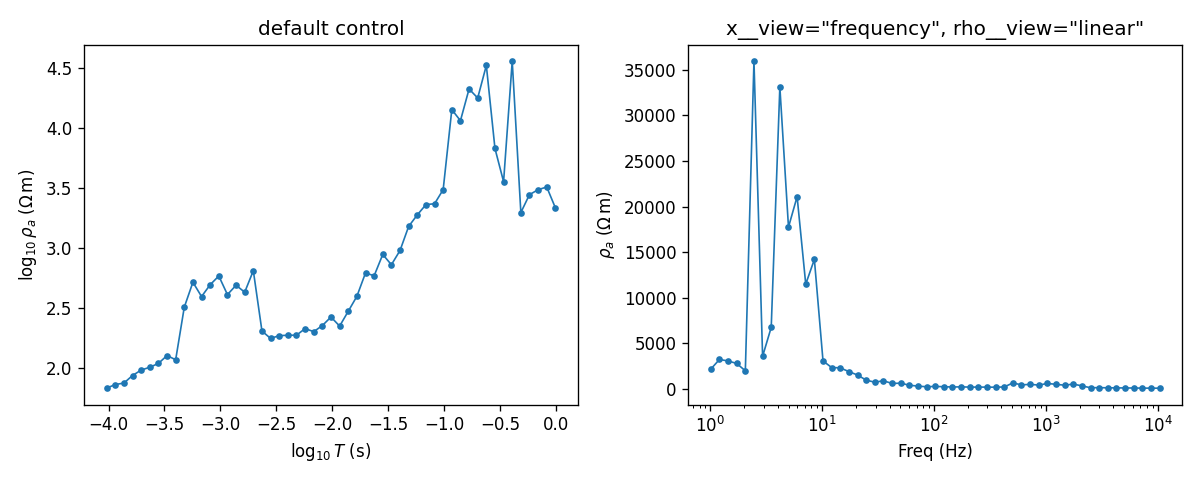
Same station, same 40-odd points either way. The left panel’s log-log
view makes the whole sounding’s frequency dependence legible; the
right panel’s linear resistivity axis makes only the two highest
peaks visible and flattens everything below about 5000 Ω·m into a
thin band along the bottom. Use "linear" deliberately – when a
collaborator specifically expects it – not as a default.#
1.10.3. Frequency Axis Control#
FrequencyAxisControl picks what the x-axis
of a 1-D sounding plot actually shows – period or frequency, log10 or
raw – and separately reports whether the axis itself should use log
scaling:
>>> PYCSAMT_CONTROL.x.transform(freq[:3])
array([-4.01703334, -3.93986854, -3.86266795])
>>> PYCSAMT_CONTROL.x.label()
'$\\log_{10}T$ (s)'
>>> PYCSAMT_CONTROL.x.use_log_scale()
False

>>> configure_control(x__view="frequency")
>>> PYCSAMT_CONTROL.x.transform(freq[:3])
array([10400.,  8707.,  7289.])
>>> PYCSAMT_CONTROL.x.label()
'Freq (Hz)'
>>> PYCSAMT_CONTROL.x.use_log_scale()
True
>>> reset_control()
That last pair is the detail easy to get wrong writing a custom plot
function: "log10_period" and "log10_frequency" already return
log10-transformed values, so
use_log_scale() reports
False for them – calling ax.set_xscale("log") on top of
already-logged data would log it twice. "period" and "frequency"
return raw values instead, so use_log_scale() reports True for
those – the axis needs the log scale because the data itself is not
pre-transformed. Always call use_log_scale() rather than assuming an
axis needs (or doesn’t need) log scaling from the view name alone.
1.10.4. Configuring And Sharing Styles#
configure_control() and
PYCSAMT_CONTROL.context()
follow the same dotted-path pattern as every other family on this page –
phase__range, rho__view, x__view – and the context manager
restores all three controls together on exit, even if the block raises:
>>> PYCSAMT_CONTROL.rho.view, PYCSAMT_CONTROL.x.view
('log10', 'log10_period')

>>> with PYCSAMT_CONTROL.context(rho__view="linear", x__view="frequency"):
...     PYCSAMT_CONTROL.rho.view, PYCSAMT_CONTROL.x.view
('linear', 'frequency')

>>> PYCSAMT_CONTROL.rho.view, PYCSAMT_CONTROL.x.view
('log10', 'log10_period')
Multi-Station Diagnostic Panels’s “Use Display Control” section shows
this same context manager wrapped around a real
plot_raw_sites_1d() call, reading back the
resulting axis labels and limits – the version of this pattern to reach
for when the control should apply to an existing plotting function rather
than a hand-written one like the panel above.
1.10.5. Next Steps#
Multi-Station Diagnostic Panels for
PYCSAMT_CONTROLwired into a real, complete plotting function call.API configuration for how the view-controls family fits alongside every other
pycsamt.apiconfiguration family.Plot Styles for the colour and marker side of the same figures – view controls decide what values are shown, Plot Styles decides how they look.