
6. Impedance Tensor#
The impedance tensor is the central frequency-domain response used in MT, AMT, and many CSAMT processing workflows. It relates horizontal electric fields to horizontal magnetic fields at each station and each frequency. In pyCSAMT, the tensor is also the bridge between raw field measurements, apparent resistivity/phase products, tensor diagnostics, static-shift correction, dimensionality analysis, and inversion input files.
This page explains the notation, physical meaning, and practical interpretation of the impedance tensor as used throughout pyCSAMT, continuing from the family-of-methods picture in CSAMT, AMT, and MT Overview and the numeric constants in Physical And Geodetic Constants.
6.1. Role In MT, AMT, And CSAMT#
For natural-source MT and AMT, the working assumption is that the incident source field behaves approximately as a plane-wave field over the survey area. Under that assumption, the horizontal electric field vector \(\mathbf{E}_h\) is related to the horizontal magnetic field vector \(\mathbf{H}_h\) by a complex frequency-dependent tensor:
Written component by component:
Each entry \(Z_{ij}\) is complex. Its amplitude controls apparent resistivity, and its phase describes the lag between electric and magnetic fields. Because \(\mathbf{Z}\) varies with frequency, it encodes how subsurface conductivity is sampled at different EM diffusion scales.
For CSAMT, the same impedance-style quantities may be computed from
controlled-source measurements, but the interpretation must account for
source-receiver geometry. In a far-field CSAMT regime, MT-like impedance
interpretation is often useful. In near-field or transition-zone regimes,
source overprint and shadow effects may make a simple impedance
interpretation misleading – see CSAMT, AMT, and MT Overview for the
classify_field_zones() diagnostic that makes
that distinction concrete.
6.2. Coordinate Convention#
The tensor notation depends on a coordinate system. pyCSAMT follows the usual two-horizontal-axis convention:
\(x\): first horizontal axis, commonly north or profile-aligned;
\(y\): second horizontal axis, commonly east or cross-profile;
\(z\): positive vertical axis by the convention used in the input data or processing workflow.
The component \(Z_{xy}\) maps \(H_y\) into \(E_x\), while \(Z_{yx}\) maps \(H_x\) into \(E_y\). Component labels are therefore not just names; they are tied to the data rotation and survey orientation.
In pyCSAMT code, a tensor stack is stored as an array with shape
(n_freq, 2, 2):
Component |
Array index |
Meaning |
|---|---|---|
\(Z_{xx}\) |
|
\(H_x\) contribution to \(E_x\). |
\(Z_{xy}\) |
|
\(H_y\) contribution to \(E_x\). |
\(Z_{yx}\) |
|
\(H_x\) contribution to \(E_y\). |
\(Z_{yy}\) |
|
\(H_y\) contribution to \(E_y\). |
This convention is used by pycsamt.z.z.Z,
pycsamt.seg.ops.z_to_rho_phi(), and tensor-related processing steps.
6.3. Complex Numbers And Phase#
Each impedance component can be written in rectangular form:
or polar form:
The component phase is:
In implementation, this is normally computed with a quadrant-aware function
such as atan2 or np.angle. pyCSAMT reports phase in degrees
for user-facing apparent resistivity/phase products.
6.4. Apparent Resistivity#
The apparent resistivity associated with a component \(Z_{ij}\) is:
where \(\mu_0\) is magnetic permeability of free space and \(\omega = 2 \pi f\).
With \(\mu_0 = 4\pi \times 10^{-7}\) H/m, this is commonly written in the numerical form used by pyCSAMT’s internal utilities:
when \(f\) is in Hz and the impedance units follow the legacy Zonge-style convention (apparent resistivity’s glossary entry gives the same shortcut). The inverse relationship is:
This is why pyCSAMT can reconstruct complex impedance from apparent resistivity and phase:
(6) and (7) are algebraically the same
physics under a unit conversion – Physical And Geodetic Constants derives exactly this
equivalence from RHO_FACTOR and ZONGE_RHO_FACTOR. What is easy to
miss is that pyCSAMT does not apply that conversion automatically
between its own two resistivity code paths. pycsamt.seg.ops.z_to_rho_phi()
implements (6) directly (\(\rho_a = |Z|^2 \cdot
\mathrm{RHO\_FACTOR}/f\)), while pycsamt.z.z.Z – built on
pycsamt.z.resphase.ResPhase, the container actually populated by
the EDI, Zonge, and Jones readers – implements (7)
directly (\(\rho_a = 0.2\,|Z|^2/f\)). Feeding the same raw z array
to both, without converting units first, does not raise an error; it
silently returns two resistivities that differ by a fixed factor:
>>> import numpy as np
>>> from pycsamt.seg.ops import z_to_rho_phi
>>> from pycsamt.z.z import Z
>>> from pycsamt.constants import RHO_FACTOR, ZONGE_RHO_FACTOR
>>> freq = np.array([10.0, 1.0, 0.1])
>>> z = np.zeros((freq.size, 2, 2), dtype=complex)
>>> z[:, 0, 1] = 1.0 + 1.0j
>>> z[:, 1, 0] = -1.0 - 1.0j
>>> rho_si, phase_si = z_to_rho_phi(z, freq)
>>> rho_si[:, 0, 1]
array([  25330.29591058,  253302.95910584, 2533029.59105844])
>>> zc = Z(z_array=z, freq=freq)
>>> zc.res_xy
array([0.04, 0.4 , 4.  ])
>>> round(float((rho_si[:, 0, 1] / zc.res_xy)[0]), 2)
633257.4
>>> round(RHO_FACTOR / ZONGE_RHO_FACTOR, 2)
633257.4
The ratio is not a coincidence or a rounding artefact – it is exactly
RHO_FACTOR / ZONGE_RHO_FACTOR, confirmed above to six significant
figures both ways. Unlike the skin-depth constant duplication in
CSAMT, AMT, and MT Overview (four numbers agreeing to a part in ten
thousand), this is a genuine convention split: z_to_rho_phi() expects
\(Z\) already in SI ohms, while Z/ResPhase expect the
legacy field-style scaling baked into the 0.2 factor, and pyCSAMT has no
code path that converts between the two automatically. In practice this
rarely bites, because z_to_rho_phi()/rho_phi_to_z() are
lightweight standalone helpers not currently called anywhere in the
EDI/Zonge/Jones ingestion pipeline – but it means the two are only
comparable after an explicit conversion like the one worked out in
Physical And Geodetic Constants, never by passing the same array to both.
Apparent resistivity is not the true resistivity at one depth. It is the resistivity of a uniform half-space that would produce the same component response at that frequency. In layered or laterally varying Earth structures, one frequency samples a broad sensitivity volume rather than a single point.
6.5. Diagonal And Off-Diagonal Components#
The four tensor components carry different interpretation weight depending on Earth dimensionality and coordinate rotation.
For a simple 1-D Earth, after using a consistent horizontal coordinate system, the ideal tensor has zero diagonal terms and antisymmetric off-diagonal terms:
For a 2-D Earth rotated into strike coordinates, the diagonal terms are also ideally zero, while \(Z_{xy}\) and \(Z_{yx}\) represent the two principal modes:
The exact assignment of TE mode and TM mode depends on coordinate convention and strike orientation, so pyCSAMT documentation prefers explicit component names unless a workflow has clearly defined the strike frame.
For a 3-D Earth, all four entries may be significant:
Large diagonal components, inconsistent strike estimates, strong tipper behavior, or high skew values can indicate that a simple 1-D or 2-D interpretation is not reliable. The next section builds exactly these three cases ((10), (11)) numerically, rather than only asserting how they behave under rotation.
6.6. Tensor Rotation#
Rotating the horizontal coordinate system changes the impedance tensor. In pyCSAMT, the rotation rule used by SEG-style operations is:
where:
The same angle can be applied to all frequencies, or a frequency-dependent
angle can be used when the processing workflow allows it. In pyCSAMT this
operation appears in functions such as
pycsamt.seg.ops.rotate_impedance() and tensor pipeline steps.
Rotation is not cosmetic. A genuinely 2-D tensor ((11), unequal \(Z_{\mathrm{TE}}\) and \(Z_{\mathrm{TM}}\)) picks up diagonal terms as soon as it is rotated away from its native strike, while a perfectly 1-D tensor ((10)) does not change at all – rotating an isotropic response cannot manufacture a preferred direction that was never there:
>>> import numpy as np
>>> from pycsamt.seg.ops import rotate_impedance
>>> z1d = np.zeros((1, 2, 2), dtype=complex)
>>> z1d[0, 0, 1] = 1.0 + 1.0j
>>> z1d[0, 1, 0] = -1.0 - 1.0j
>>> z2d = np.zeros((1, 2, 2), dtype=complex)
>>> z2d[0, 0, 1] = 1.0 + 1.0j   # Z_TE at native strike
>>> z2d[0, 1, 0] = 3.0 + 0.5j   # Z_TM at native strike
>>> det0 = z2d[0, 0, 0] * z2d[0, 1, 1] - z2d[0, 0, 1] * z2d[0, 1, 0]
>>> det0
(-2.5-3.5j)
>>> z_rot20 = rotate_impedance(z2d, theta_deg=20.0)
>>> z_rot20.shape
(2, 2)
>>> np.allclose(np.linalg.det(z_rot20), det0)
True
>>> np.allclose(np.trace(z_rot20), 0.0)
True
>>> np.allclose(z_rot20[0, 1] - z_rot20[1, 0], z2d[0, 0, 1] - z2d[0, 1, 0])
True
>>> angles = np.linspace(-90, 90, 181)
Note that z_rot20.shape is (2, 2), not (1, 2, 2) –
rotate_impedance() squeezes any length-1 axis in its result, including
the frequency axis when only one frequency is given. Index the rotated
matrix directly rather than adding an extra [0].
The three True results above are not particular to this example: the
determinant, the trace, and the antisymmetric part \(Z_{xy}-Z_{yx}\)
are each exactly invariant under (13) for any tensor,
for three different linear-algebra reasons – \(\det(\mathbf{R}\mathbf{Z}\mathbf{R}^T)
=\det(\mathbf{Z})\) because \(\det(\mathbf{R})=1\); the trace is
invariant under any orthogonal similarity transform; and a pure rotation
preserves a 2-D antisymmetric matrix exactly. What does change is visible
directly: the two diagonal terms grow individually away from strike even
though their sum never does.
 1import numpy as np
 2import matplotlib.pyplot as plt
 3from pycsamt.seg.ops import rotate_impedance
 4
 5angles = np.linspace(-90, 90, 181)
 6
 7z1d = np.zeros((1, 2, 2), dtype=complex)
 8z1d[0, 0, 1] = 1.0 + 1.0j
 9z1d[0, 1, 0] = -1.0 - 1.0j
10zr1 = rotate_impedance(z1d, theta_deg=angles)
11diag1 = np.abs(zr1[:, 0, 0]) + np.abs(zr1[:, 1, 1])
12
13z2d = np.zeros((1, 2, 2), dtype=complex)
14z2d[0, 0, 1] = 1.0 + 1.0j
15z2d[0, 1, 0] = 3.0 + 0.5j
16zr2 = rotate_impedance(z2d, theta_deg=angles)
17diag2 = np.abs(zr2[:, 0, 0]) + np.abs(zr2[:, 1, 1])
18
19fig, ax = plt.subplots(1, 1, figsize=(7.0, 4.2))
20ax.plot(angles, diag2, color="#1f77b4", lw=2.2, label="2-D tensor (Zxy != Zyx)")
21ax.plot(angles, diag1, color="#d62728", lw=2.2, ls="--", label="1-D tensor (Zxy = -Zyx)")
22ax.axvline(0.0, color="0.5", lw=1.0, ls=":")
23ax.set(xlabel=r"Rotation angle $\theta$ (degrees)",
24       ylabel=r"$|Z_{xx}| + |Z_{yy}|$",
25       title="Diagonal growth under rotation")
26ax.legend(fontsize=9)
27ax.grid(True, alpha=0.3)
28fig.tight_layout()
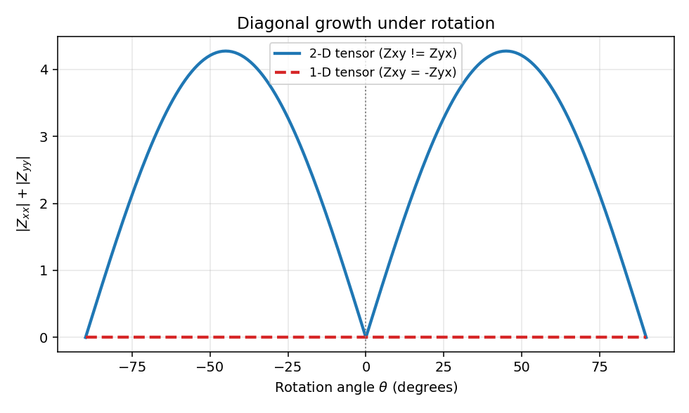
The 2-D tensor’s diagonal grows to a maximum near \(\pm 45^\circ\) and returns to zero every \(90^\circ\) – rotating by a quarter turn swaps the axes and lands on another zero-diagonal frame with TE and TM exchanged. The 1-D tensor stays at floating-point zero for every angle: there is no strike to find because the response has none.#
6.7. Strike, Principal Directions, And Ambiguity#
In 2-D interpretation, the goal is often to rotate the tensor into a coordinate frame aligned with geological strike. In a perfect 2-D case, there exists an angle \(\theta_s\) such that the diagonal terms are minimized and the off-diagonal modes are physically interpretable. That angle can be found directly by scanning (13) over a range of trial angles and keeping the one with the smallest diagonal magnitude – exactly the curve plotted above, read off numerically instead of by eye:
>>> z_scan = rotate_impedance(z2d, theta_deg=angles)
>>> diag_mag = np.abs(z_scan[:, 0, 0]) + np.abs(z_scan[:, 1, 1])
>>> round(float(angles[np.argmin(diag_mag)]), 1)
0.0
>>> round(float(diag_mag.min()), 6)
0.0
The recovered strike, \(0.0^\circ\), matches the frame the synthetic tensor was built in – as expected, since \(\mathtt{z2d}\) was constructed already in strike coordinates. Real data will not return an exact zero; the same grid search still applies, but the achievable minimum reflects noise, 3-D structure, and distortion rather than floating-point precision.
In practice, strike estimation is ambiguous because:
MT strike often has a \(90^\circ\) ambiguity, visible in the figure above as the second zero-diagonal frame near the scan’s edges;
near-surface distortion can affect impedance components;
different frequency bands may sample different structures;
3-D geology may not have one stable strike;
CSAMT source geometry can bias component behavior.
pyCSAMT strike and tensor diagnostics should therefore be treated as evidence, not as automatic truth. A robust workflow compares strike estimates with geology, station layout, tipper vectors, phase tensors, residuals, and inversion behavior.
6.8. Phase Tensor#
The phase tensor is a distortion-resistant diagnostic constructed from the real and imaginary parts of the impedance tensor. Let:
where \(\mathbf{X} = \operatorname{Re}(\mathbf{Z})\) and \(\mathbf{Y} = \operatorname{Im}(\mathbf{Z})\). The phase tensor is:
The defining property that makes (16) useful is easy to lose sight of algebraically but obvious numerically: \(\mathbf{\Phi}\) is a real-valued matrix, even though \(\mathbf{Z}\) is complex, because it is built from the product of two real matrices:
>>> X, Y = z2d[0].real, z2d[0].imag
>>> Phi = np.linalg.inv(X) @ Y
>>> Phi
array([[0.16666667, 0.        ],
       [0.        , 1.        ]])
>>> Phi.dtype == np.dtype("float64")
True
It describes the phase relationship independent of galvanic amplitude scaling under common distortion assumptions. Phase tensor ellipses are used to inspect:
dimensionality;
strike direction;
phase anisotropy;
skew or 3-D behavior;
station-to-station consistency;
period-dependent structural changes.
The phase tensor does not remove every problem. It does not make poor data good, it does not eliminate inductive 3-D effects, and it does not replace model-based interpretation. It is a diagnostic that helps decide which processing and inversion assumptions are defensible.
Dimensionality, Distortion, And The Phase Tensor derives the orientation angle \(\alpha\) and skew angle \(\beta\) behind these ellipses in full, including a real bug this documentation project found in the angle formulas, and uses them to classify 1-D/2-D/3-D behavior station by station on real data.
6.9. Skew And Dimensionality#
Skew metrics summarize departures from simple dimensionality. Different families of skew exist, and they should not be confused with the simple linear-algebra skew \(Z_{xy} - Z_{yx}\) used as a rotation invariant above. A standard distortion-tolerant choice is Bahr skewness, built from the symmetric and antisymmetric combinations of \(\mathbf{Z}\):
pycsamt.emtools.skew.bahr_skewness() implements
(17)/(18) directly. Run on the same
\(\mathtt{z2d}\) tensor before and after the \(20^\circ\) rotation
used above, it returns the identical value both times – Bahr skewness is a
rotational invariant by construction, just like the determinant and trace
already confirmed:
>>> from pycsamt.emtools.skew import bahr_skewness
>>> eta0 = bahr_skewness(z2d)
>>> eta20 = bahr_skewness(z_rot20[np.newaxis, ...])
>>> round(float(eta0[0]), 6), round(float(eta20[0]), 6)
(0.482573, 0.482573)
As a practical guide:
low skew over a continuous band supports 1-D or 2-D modelling assumptions;
high skew may indicate 3-D structure, distortion, bad data, or source effects;
isolated high-skew frequencies may reflect noise or processing artifacts;
skew should be compared with phase tensor, tipper, and residual plots.
pyCSAMT pipeline steps can mask, select, or close gaps in low-skew frequency bands. Those operations should be documented in the workflow report because they affect which data enter inversion. Dimensionality, Distortion, And The Phase Tensor also covers the Groom-Bailey galvanic-distortion decomposition, a more complete alternative to Bahr skewness when a real distortion matrix (not just a scalar skew) needs to be estimated and removed.
6.10. Tipper And Vertical Magnetic Field#
The impedance tensor uses horizontal electric and magnetic fields. The vertical magnetic field is commonly described with the tipper:
The tipper vector \(\mathbf{T} = [T_x, T_y]\) is sensitive to lateral conductivity contrasts. Large tipper magnitudes or coherent induction vectors often indicate 2-D or 3-D structure. In a laterally uniform 1-D Earth, the ideal tipper is zero.
Under horizontal rotation, pyCSAMT rotates the tipper as a vector:
Because (20) is a plain vector rotation (not the two-sided (13) used for the tensor), its Euclidean norm \(\sqrt{|T_x|^2+|T_y|^2}\) is preserved exactly – rotation redistributes the tipper between components without changing its overall magnitude:
>>> from pycsamt.seg.ops import rotate_tipper
>>> t = np.array([[0.3 + 0.1j, 0.05 - 0.02j]])  # Tx, Ty at one frequency
>>> t_rot = rotate_tipper(t, theta_deg=30.0)
>>> t_rot.shape
(2,)
>>> norm_before = np.hypot(abs(t[0, 0]), abs(t[0, 1]))
>>> norm_after = np.hypot(abs(t_rot[0]), abs(t_rot[1]))
>>> round(float(norm_before), 6) == round(float(norm_after), 6)
True
Tipper plots are especially useful when deciding whether a 2-D profile orientation is plausible. If induction vectors suggest strong off-profile structure, a 2-D inversion may still fit the data numerically but be geologically misleading.
6.11. Error Propagation#
Impedance estimates should be interpreted with uncertainty. If \(\Delta Z_{ij}\) is an absolute component uncertainty, then the relative amplitude error is approximately:
Because apparent resistivity depends on \(|Z|^2\), the relative resistivity error is approximately twice the relative impedance-amplitude error:
Phase uncertainty depends on the relative size of the real and imaginary
parts and becomes unstable when the impedance amplitude is very small.
pyCSAMT carries absolute z_err arrays when available and propagates them
to resistivity and phase through the pycsamt.z.resphase.ResPhase
and pycsamt.z.z.Z containers.
Error information matters for:
deciding whether a curve feature is real or noise;
weighting inversion data;
masking unstable frequencies;
comparing observed and predicted responses;
judging whether an apparent dimensionality feature is significant.
6.12. Static Shift And Galvanic Distortion#
Static shift is a near-surface galvanic distortion that multiplies apparent resistivity without changing phase in the simplest approximation. It is not primarily an impedance phase problem; it is an amplitude scaling problem.
If \(g_x\) and \(g_y\) are real electric-field gains, a simplified distortion model can be written:
where \(\mathbf{C}\) is a real distortion matrix. Then:
Because \(\mathbf{C}\) is real, left-multiplying by it rescales each row of \(\mathbf{Z}\) without touching phase – exactly the “amplitude only” behavior the name implies:
>>> C = np.diag([1.4, 0.6])  # real, positive static-shift gains
>>> z_true = z1d[0]
>>> z_obs = C @ z_true
>>> np.round(np.angle(z_obs, deg=True), 6)
array([[   0.,   45.],
       [-135.,    0.]])
>>> np.round(np.angle(z_true, deg=True), 6)
array([[   0.,   45.],
       [-135.,    0.]])
>>> np.abs(z_obs) / np.abs(z_true)
array([[nan, 1.4],
       [0.6, nan]])
Phase is identical before and after distortion (the nan entries above
are the zero diagonal, 0/0); only the off-diagonal amplitudes are
scaled, by \(g_x=1.4\) and \(g_y=0.6\) respectively. This is why
static shift can move apparent resistivity curves up or down without
producing an equivalent phase shift. The detailed interpretation is covered
in Static Shift, but the tensor view is important: correcting static
shift changes amplitudes before apparent resistivity is interpreted or
inverted.
6.13. Determinant And Other Invariants#
Tensor invariants are scalar combinations of \(\mathbf{Z}\) that can be useful for plotting, comparison, or quality control. Common examples are:
and the Frobenius norm:
(25) and (26) are exactly the two invariants
already confirmed under rotation in the worked example above – “invariant”
here is not a qualitative claim, it is the np.allclose(..., True) result
from that block. pyCSAMT exposes such quantities through the
pycsamt.z.z.Z container (.trace, .det, .norm). They are
helpful diagnostics, but they are not a replacement for understanding tensor
orientation, uncertainty, and dimensionality.
6.14. Practical Component Choices#
Many workflows focus on off-diagonal components because they are dominant for ideal 1-D and 2-D MT responses. Typical choices include:
Choice |
Use |
Caution |
|---|---|---|
\(Z_{xy}\) |
One principal off-diagonal response. |
Meaning depends on coordinate frame and strike convention. |
\(Z_{yx}\) |
The other principal off-diagonal response. |
Often has opposite sign or phase convention relative to \(Z_{xy}\). |
Determinant response |
Rotation-tolerant summary response for some quick-look plots. |
Can hide mode-specific behavior and poor component quality. |
Average off-diagonal response |
Simple 1-D-style sounding or quick QC. |
Can blur TE/TM differences and 2-D structure. |
Phase tensor quantities |
Dimensionality and strike diagnostics. |
Not a replacement for amplitude-sensitive inversion. |
The safest documentation and reports should always state the component,
invariant, and resistivity convention used. “Apparent resistivity”
alone is incomplete; say \(\rho_{a,xy}\), \(\rho_{a,yx}\),
determinant apparent resistivity, or the exact product used – and, per the
worked example above, whether it came from z_to_rho_phi()’s SI
convention or Z’s legacy Zonge-style convention, since the two are
not interchangeable on the same raw array.
6.15. pyCSAMT Containers And Utilities#
Several pyCSAMT modules use the tensor concepts directly.
Object or function |
Role |
|---|---|
High-level impedance tensor container with shape |
|
Converts between complex impedance and apparent resistivity/phase using (7), including error propagation. |
|
|
Stores complex tipper components, rotations, amplitudes, phases, and arrow metrics. |
|
Computes component-wise apparent resistivity and phase from impedance and frequency using the SI convention ((6)) – not currently wired into the EDI/Zonge/Jones ingestion pipeline, see the worked comparison above. |
|
Reconstructs complex impedance from apparent resistivity, phase, and
frequency (same SI convention as |
|
Applies \(\mathbf{Z}' = \mathbf{R}\mathbf{Z}\mathbf{R}^T\); squeezes length-1 axes in its output (see the rotation example above). |
|
Rotates tipper vectors consistently with the horizontal coordinate frame; same squeeze behavior for a single frequency. |
|
Computes the rotation-invariant Bahr skew ((18)) used for dimensionality screening. |
6.16. Quality Control Questions#
Before using impedance tensors in inversion or interpretation, ask:
Are frequencies positive, sorted, and consistent across stations?
Are tensor components in the expected coordinate convention?
Were rotations applied, and are the rotation angles recorded?
Are \(Z_{xy}\) and \(Z_{yx}\) internally consistent?
Are diagonal terms physically meaningful, or dominated by noise?
Are phase curves smooth enough to trust?
Are apparent resistivity shifts consistent with static shift?
Does the phase tensor suggest 1-D, 2-D, or 3-D behavior?
Do tipper vectors support the selected profile orientation?
Are errors available for inversion weighting?
Which resistivity convention (SI or legacy Zonge-style) produced the numbers being compared?
6.17. Interpretation Pitfalls#
Common tensor mistakes include:
treating the tensor as four independent curves with no coordinate context;
rotating data without documenting the angle and sign convention;
assuming diagonal components are always noise;
assuming off-diagonal antisymmetry guarantees a 1-D Earth;
averaging \(Z_{xy}\) and \(Z_{yx}\) before checking mode behavior;
interpreting apparent resistivity amplitudes without static-shift review;
trusting a low RMS inversion while ignoring tensor residual patterns;
using CSAMT impedance-style products without checking source effects;
mixing
z_to_rho_phi()’s SI convention withZ’s legacy Zonge-style convention on the same raw impedance values.
6.18. Connection To Later Workflows#
The impedance tensor feeds directly into:
Static Shift, because galvanic distortion affects amplitude;
Inversion Concepts, because inversion fits impedance, resistivity/phase, or transformed tensor products;
Pipeline Steps, because tensor cleanup, skew gates, rotations, and dimensionality diagnostics are registered pipeline steps;
Correct Static Shift, because practical correction begins with apparent resistivity and phase inspection;
pycsamt.z, because the public tensor containers are documented in the API reference.
6.19. References#
This page follows standard MT tensor notation and the implementation conventions in pyCSAMT. Relevant background references are collected in References, especially [WardHohmann1988], [deGrootHedlin1990], and [Kelbert2014].