
8. Static Shift#
Static shift is a near-surface galvanic distortion that moves apparent resistivity curves up or down without producing the same change in phase. It is one of the most important practical problems in MT, AMT, and CSAMT interpretation because it can create false shallow resistivity contrasts and can bias inversion starting models, pseudo-sections, and final sections.
In the simplest case, a station sits above a small shallow conductor or resistor. The shallow body distorts the electric field measured at the surface. The magnetic field and phase relationship may remain comparatively stable, but the electric-field amplitude is scaled. Because apparent resistivity is proportional to impedance amplitude squared, a modest electric-field scaling can become a large apparent-resistivity shift.
This page explains the physics, diagnostics, and pyCSAMT correction workflow
for static shift, continuing from the amplitude/phase notation in
Impedance Tensor. Every number below is a real result from the
bundled 28-station L18PLT AMT survey (data/AMT/WILLY_DATA/L18PLT), not a
synthetic stand-in. The companion tutorial
Correct Static Shift shows the practical API calls in a
full workflow context.
8.1. Why Static Shift Happens#
MT, AMT, and far-field CSAMT interpretation assume that the measured horizontal electric and magnetic fields represent regional electromagnetic induction. Near the surface, however, small resistivity heterogeneities can accumulate charge and distort the electric field. This is called galvanic distortion because it is controlled by current channelling and charge build-up in shallow conductivity contrasts.
Common causes include:
conductive clay lenses;
dry resistive boulders or lateritic caps;
weathered fracture zones;
shallow groundwater salinity changes;
cultural conductors such as fences, pipes, cables, and grounding systems;
local topographic or contact effects near electrodes.
The important feature is scale. Static shift is usually caused by structures that are shallow and small compared with the induction scale of the periods or frequencies being interpreted. They can strongly affect local electric field amplitudes while leaving the deeper induction response broadly intact.
8.2. Scale Factor Notation#
For a simple scalar static shift, the observed apparent resistivity at one station can be written as
where \(s_{\rho}\) is a positive station-dependent scale factor. In logarithmic units this becomes an additive offset:
The offset \(\Delta_{\rho}\) is approximately constant with frequency when the distortion is truly static.
For impedance amplitude, the relation is
and because apparent resistivity is proportional to \(|Z|^2\),
pyCSAMT correction tables therefore report both fac_rho and fac_z.
The impedance tensor is corrected with fac_z because the stored field
quantity is impedance, while apparent resistivity curves respond with the
square of that factor. (4) is not just an algebra
identity here – it is exactly what pycsamt.emtools.ss.estimate_ss_ama()
returns for every station, station 18-007U of the L18PLT survey being the
most strongly shifted:
>>> import numpy as np
>>> from pycsamt.api import read_edis
>>> from pycsamt.emtools.ss import estimate_ss_ama
>>> sites = read_edis("data/AMT/WILLY_DATA/L18PLT", progress=False).collection
>>> len(sites)
28
>>> factors = estimate_ss_ama(
...     sites, sort_by="lon", half_window=3, weights="tri", max_skew=6.0, api=True,
... )
>>> row = factors.loc[factors["station"] == "18-007U"].iloc[0]
>>> round(float(row["fac_rho"]), 6)
21.819976
>>> round(float(row["fac_z"]), 6)
4.671186
>>> round(float(np.sqrt(row["fac_rho"])), 6)
4.671186
fac_z and sqrt(fac_rho) agree to six decimal places because they are
computed from the same underlying \(\Delta_\rho\) estimate, not fit
independently.
8.3. Tensor View#
The scalar model is useful, but real galvanic distortion can mix impedance components. A common distortion model is
where \(\mathbf{C}\) is a real, frequency-independent distortion matrix – the same relation as (24) in Impedance Tensor, where it was verified numerically that a real \(\mathbf{C}\) leaves phase untouched. Static shift is the amplitude-scaling part of this broader distortion problem. Twist, shear, anisotropy, and component mixing can also occur.
This is why static-shift correction should be paired with tensor diagnostics. If phase tensor skew, induction vectors, or component residuals suggest strong 3-D mixing, a simple station-level amplitude factor may not be enough. See Impedance Tensor for the impedance and phase-tensor background, and Dimensionality, Distortion, And The Phase Tensor for the full Groom-Bailey decomposition of \(\mathbf{C}\) into twist, shear, and anisotropy – including a real, honest example of the correction making some stations’ diagonal terms worse rather than better, which is exactly the kind of 3-D mixing this section warns about.
8.4. Why Phase Is Less Affected#
Apparent resistivity uses impedance amplitude:
The impedance phase uses the ratio of imaginary and real parts:
If the distortion is a real scalar multiplier, both \(\mathrm{Re}(Z)\) and \(\mathrm{Im}(Z)\) are scaled by the same factor. The amplitude changes, but the phase ratio does not:
Continuing the same station, correction changes \(\rho_{a,xy}\) by the
full fac_rho=21.82 factor while leaving phase bit-for-bit identical –
not approximately equal, exactly equal, since (8)
holds to floating-point precision for a real fac_z:
>>> from pycsamt.emtools.ss import correct_ss_ama
>>> corrected = correct_ss_ama(
...     sites, sort_by="lon", half_window=3, weights="tri", inplace=False,
... )
>>> raw = next(s for s in sites if s.station == "18-007U")
>>> cor = next(s for s in corrected if s.name == "18-007U")
>>> np.allclose(raw.Z.phase_xy, cor.phase[:, 0, 1])
True
>>> np.allclose(raw.Z.res_xy, cor.rho[:, 0, 1])
False
>>> ratio = cor.rho[:, 0, 1] / raw.Z.res_xy
>>> round(float(ratio.min()), 6), round(float(ratio.max()), 6)
(21.819976, 21.819976)
The resistivity ratio is constant across every one of the station’s 53
frequencies and matches fac_rho exactly – this is the classic
diagnostic pattern: apparent resistivity curves are offset relative to
nearby stations, while phase curves remain smooth and geologically
consistent. If phase is also strongly distorted, the problem may not be
simple static shift.
8.5. Static Shift Versus Near-Surface Effect#
pyCSAMT makes an important operational distinction between:
static shift - a frequency-independent multiplicative shift of the whole apparent-resistivity curve;
near-surface effect - a frequency-dependent distortion, often strongest at high frequencies, caused by shallow inhomogeneities or source/electrode effects.
Static shift can often be corrected by estimating a station-level amplitude factor. Frequency-dependent near-surface effects should not be “fixed” with a single static factor because the curve shape itself has changed. In that case, better options include masking the contaminated band, improving processing, using 2-D/3-D inversion, or explicitly modelling the near-surface structure.
In pycsamt.emtools.ss, near-surface distortion classification uses
three station diagnostics:
ss_delta_log10- the median log10 apparent-resistivity offset relative to an AMA spatial trend;ns_index- a high-frequency versus low-frequency residual spread ratio;gradient_delta- the difference between high-frequency and low-frequency log-log slopes.
The classification vocabulary is:
Class |
Meaning |
Suggested response |
|---|---|---|
|
No strong static or near-surface flag. |
Keep the station; inspect normally. |
|
Frequency-independent offset dominates. |
Apply static-shift correction and compare before/after. |
|
Frequency-dependent high-frequency distortion dominates. |
Mask contaminated band or use modelling/inversion that can represent shallow structure. |
|
Both offset and frequency-dependent distortion are present. |
Correct cautiously; preserve diagnostics and consider excluding unstable bands. |
Running pycsamt.emtools.ss.detect_near_surface() on the same 28
stations, at its documented default thresholds, is a useful reminder that
real classification results are rarely evenly spread across all four
labels:
>>> from pycsamt.emtools.ss import detect_near_surface
>>> classes = detect_near_surface(
...     sites, f_split=1.0, ns_threshold=2.0, ss_threshold=0.1,
...     sort_by="lon", half_window=3, weights="tri", api=True,
... )
>>> classes["distortion_type"].value_counts().to_dict()
{'static': 24, 'clean': 2}
Every classified station in this survey is either clean or static –
none crosses the near_surface or mixed thresholds at these settings.
That is a property of this line and these thresholds, not a guarantee;
a survey with strong high-frequency cultural noise or shallow karst would
be expected to populate the other two classes. As with estimate_ss_ama
above, only 26 of the 28 stations appear here – see the masked-station note
in the AMA API section below before assuming every station gets classified.
8.6. How It Appears In Profiles#
In a profile, static shift usually appears as a station-level vertical jump in apparent resistivity. The shifted curve may preserve the same shape as neighbouring curves but sit consistently higher or lower.
Look for:
one or a few stations offset from a smooth spatial trend;
apparent resistivity discontinuities without corresponding phase changes;
TE and TM apparent resistivity shifts that are not matched by phase;
determinant apparent resistivity offsets near one station;
pseudo-section vertical stripes or station-centred anomalies;
shallow inversion anomalies that disappear when the station is corrected or down-weighted.
Plotting \(\Delta_\rho\) for every L18PLT station, sorted by offset, shows exactly this pattern: most stations cluster within about \(\pm 0.5\) log10 units of zero, while a handful sit well outside that band and are the stations a reviewer should look at first.
 1import matplotlib.pyplot as plt
 2
 3fac = factors.sort_values("delta_log10_rho").reset_index(drop=True)
 4colors = ["#d62728" if abs(v) > 0.8 else "#1f77b4"
 5          for v in fac["delta_log10_rho"]]
 6
 7fig, ax = plt.subplots(1, 1, figsize=(9.0, 4.0))
 8ax.bar(range(len(fac)), fac["delta_log10_rho"], color=colors)
 9ax.axhline(0.0, color="0.3", lw=1.0)
10ax.set_xticks(range(len(fac)))
11ax.set_xticklabels(fac["station"], rotation=90, fontsize=6.5)
12ax.set(ylabel=r"$\Delta_\rho = \log_{10}\rho_{a,\mathrm{obs}} - \log_{10}T_i$",
13       title="AMA static-shift offset by station (L18PLT, sorted by offset)")
14ax.grid(True, axis="y", alpha=0.3)
15fig.tight_layout()
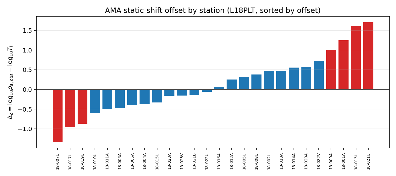
Stations 18-007U, 18-017U, and 18-019U sit furthest below the spatial trend; 18-013U and 18-021U sit furthest above it. These five are exactly the stations worth checking against field notes and phase curves before trusting the correction.#
Do not diagnose static shift from apparent resistivity alone. Compare phase, tensor skew, station quality, contact resistance, field notes, and nearby geology.
8.7. CSAMT-Specific Cautions#
CSAMT can contain both galvanic static shift and source-related effects. These should not be confused.
Static shift is station-local and approximately frequency independent in
log apparent resistivity. Source effects can be frequency dependent and may
vary systematically with transmitter distance, line geometry, and
transition from near field to far field. Shadow and
source overprint effects can change curve shape, not only level –
the same distinction classify_field_zones()
makes quantitative in CSAMT, AMT, and MT Overview.
Before applying static-shift correction to CSAMT data, check:
whether the frequency band is far-field enough for the intended interpretation;
whether the shifted station also has unusual phase behavior;
whether neighbouring stations share the same source-distance trend;
whether the apparent shift is actually a transmitter geometry effect;
whether a correction improves or damages response consistency.
See CSAMT, AMT, and MT Overview for the broader CSAMT/AMT/MT distinction.
8.8. Correction Philosophy#
Static-shift correction should be conservative. The goal is not to make every curve look smooth or pretty. The goal is to remove station-local amplitude bias while preserving regional induction structure.
Good correction practice follows these principles:
estimate factors from neighbouring stations or independent constraints;
avoid using known bad stations as references;
avoid correcting frequency-dependent curve-shape problems with one scalar;
preserve before/after plots and correction factors;
use
inplace=Falseor copy-based workflows while exploring;rerun inversion diagnostics after correction.
In hydrogeological and engineering surveys, a shallow conductor may be a real target rather than a nuisance. If a shallow body is important to the study, document whether it is being corrected as distortion or interpreted as geology.
8.9. AMA Correction In pyCSAMT#
The default pyCSAMT correction path is AMA, an adaptive moving-average spatial trend. For each station, pyCSAMT estimates a regional trend from nearby stations and compares the station’s log apparent resistivity against that trend. The shift estimate is
where \(T_i(f)\) is the spatial trend estimated from neighbouring stations at frequency \(f\).
The correction factor applied to apparent resistivity is
and the correction factor applied to impedance is
This is why the output table from pycsamt.emtools.ss.estimate_ss_ama()
contains:
Column |
Meaning |
|---|---|
|
Station identifier. |
|
Estimated log10 apparent-resistivity shift before correction. |
|
Multiplicative factor for apparent resistivity. |
|
Multiplicative factor for impedance tensor amplitudes. |
|
Number of samples used in the shift estimate. |
The full sites/factors/corrected objects built above are the
real basic API example – there is no separate synthetic version:
>>> factors.shape
(26, 5)
>>> len(sites) - len(factors)
2
>>> sorted(set(s.station for s in sites) - set(factors["station"]))
['18-024U', '18-025A']
>>> masked = next(s for s in sites if s.station == "18-024U")
>>> masked_corrected = next(s for s in corrected if s.name == "18-024U")
>>> np.allclose(masked_corrected.rho[:, 0, 1] / masked.Z.res_xy, 1.0)
True
Only 26 of the 28 stations appear in factors – max_skew=6.0 masks
individual frequencies whose phase-tensor skew is too high, and a station
disappears from the table entirely once every one of its frequencies
fails that test. Critically, correct_ss_ama does not drop those two
stations: it returns all 28, and the two masked ones come back with a
resistivity ratio of exactly 1.0 – a correction table that looks
complete but silently did nothing for them. Always cross-check
len(factors) against len(sites) before trusting a correction run;
this is the same masking mechanism documented for the K2 Stratagem survey
in Static Shift and Noise Removal.
The important parameters are:
sort_by- station order for the spatial profile, usually"lon"for east-west profiles and"lat"for north-south profiles;half_window- number of neighbouring stations on each side;weights- triangular, Gaussian, or uniform spatial weights;pband- optional period band used to estimate the factor;max_skew- optional phase-tensor skew ceiling used to avoid strongly distorted stations in the trend (and, as above, capable of masking a station out of the table entirely).
8.10. Choosing The Estimation Band#
The optional period band pband=(T_min, T_max) is important when only part
of the curve is trustworthy. A good band should:
contain enough frequencies at most stations;
avoid dead bands and noisy acquisition ranges;
avoid strong near-field CSAMT source effects;
avoid high-frequency near-surface curve-shape distortion;
represent the regional trend rather than a local target.
If the chosen band is too narrow, correction factors become unstable. If it includes contaminated frequencies, the estimated factor can absorb effects that are not static shift.
8.11. LOESS, Reference Median, and Bilateral Options#
The pipeline catalogue includes several static-shift correction styles:
Code |
Method |
Typical use |
|---|---|---|
|
AMA |
Default profile-based correction using neighbouring stations. |
|
LOESS |
Smooth spatial trend when station spacing is irregular or gradual profile-scale drift is expected. |
|
Reference median |
Correction relative to a robust median or reference response. |
|
Bilateral |
Edge-aware spatial correction that reduces smoothing across sharp station-to-station changes. |
The best method depends on survey geometry. AMA is simple and transparent.
LOESS can be better for uneven spacing. Reference median methods need a
credible reference. Bilateral filters can preserve sharp spatial transitions
but still require careful diagnostics. In pycsamt.emtools.ss, LOESS,
reference-median, and bilateral each expose an estimate_ss_* function
(estimate_ss_loess(),
estimate_ss_refmedian(),
estimate_ss_bilateral()) that returns a factor
table in the same shape as estimate_ss_ama above, applied to the data
with the shared apply_ss_factors() helper –
only AMA fuses estimation and application into one correct_ss_ama call.
8.12. Stratagem Workflow#
The Stratagem helper wraps the same idea for AMT/CSAMT survey processing:
 1from pycsamt.stratagem.process import StaticShiftCorrector
 2
 3corrector = StaticShiftCorrector(
 4    sort_by="lon",
 5    half_window=3,
 6    weights="tri",
 7    pband=None,
 8    max_skew=6.0,
 9)
10
11corrected_edis = corrector.fit(edis, copy=True).out()
12factors = corrector.factors_
copy=True preserves the original EDI objects. The correction is applied
to impedance amplitudes, so exported apparent resistivity and phase products
should be regenerated from the corrected impedance. A full real run of this
exact API on the bundled K2 Stratagem survey – including the same
per-frequency-masking gotcha found above, there affecting 12 of 86 stations
– is worked through in Static Shift and Noise Removal.
In Stratagem pipelines, static-shift correction should usually run before frequency filtering that removes many impedance samples. The code deliberately warns about this because AMA needs enough common frequency support to compare neighbouring stations.
8.13. Agent And Application Workflows#
The same correction concept is exposed in higher-level pyCSAMT workflows:
pycsamt.agents.static_shift.StaticShiftAgentcan run correction, collect summary tables, and prepare report text;the desktop application exposes AMA-style static-shift correction in the correction tools;
the web application can call the static-shift agent as part of an assisted workflow;
pycsamt.pipelineregisters static-shift steps so they can be placed between QC and inversion preparation.
These interfaces should still produce the same core evidence: correction factors, before/after curves or pseudo-sections, and enough metadata to reproduce the correction.
8.14. Before/After Interpretation#
After correction, inspect:
apparent resistivity before and after correction;
phase before and after correction;
pseudo-sections of the correction delta;
station-level correction factors;
tensor skew or phase-tensor diagnostics;
inversion residuals before and after correction.
The two L18PLT stations plotted below make this concrete: 18-007U’s curve
moves up by a constant fac_rho=21.82 and 18-001A’s moves down by
fac_rho=0.056, both parallel shifts in log-log space, while their phase
curves are unchanged (compare the left and right panels).
 1import matplotlib.pyplot as plt
 2
 3
 4def find(coll, name):
 5    for s in coll:
 6        st = getattr(s, "station", None) or getattr(s, "name", None)
 7        if st == name:
 8            return s
 9
10
11fig, axes = plt.subplots(1, 2, figsize=(10.5, 4.4))
12for name, color in [("18-007U", "#d62728"), ("18-001A", "#1f77b4")]:
13    raw = find(sites, name)
14    cor = find(corrected, name)
15    axes[0].loglog(raw.Z.freq, raw.Z.res_xy, color=color, lw=1.4, ls="--",
16                    label=f"{name} raw")
17    axes[0].loglog(raw.Z.freq, cor.rho[:, 0, 1], color=color, lw=2.2,
18                    label=f"{name} corrected")
19    axes[1].semilogx(raw.Z.freq, raw.Z.phase_xy, color=color, lw=1.4, ls="--")
20    axes[1].semilogx(raw.Z.freq, cor.phase[:, 0, 1], color=color, lw=2.2)
21
22axes[0].set(xlabel="Frequency (Hz)", ylabel=r"$\rho_{a,xy}$ ($\Omega\cdot$m)",
23            title="Apparent resistivity: raw vs AMA-corrected")
24axes[0].legend(fontsize=7.5)
25axes[0].grid(True, which="both", alpha=0.3)
26axes[1].set(xlabel="Frequency (Hz)", ylabel=r"$\phi_{xy}$ (degrees)",
27            title="Phase: raw and corrected overlap exactly")
28axes[1].grid(True, which="both", alpha=0.3)
29fig.tight_layout()
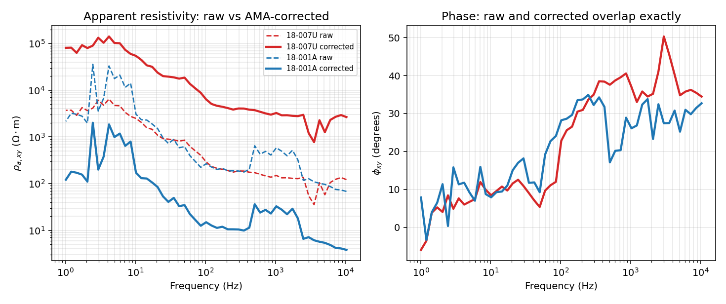
18-007U (red) is shifted up, 18-001A (blue) is shifted down; both keep their curve shape. The right panel’s dashed and solid lines lie exactly on top of each other – correction changes level, not shape.#
The correction is plausible when:
shifted apparent resistivity curves align better with neighbouring station trends;
phase remains essentially unchanged;
correction factors are not extreme;
response fits improve without creating new residual patterns;
the corrected section is geologically coherent and still honours known shallow structure.
The correction is suspicious when:
a large factor is required for many adjacent stations;
phase changes or phase residuals are also problematic;
the apparent shift is frequency dependent;
the corrected curve no longer matches nearby geology or field notes;
inversion improves globally but worsens systematically at corrected stations.
8.15. Effect On Inversion#
Static shift can strongly affect inversion. If left uncorrected, a downshift in apparent resistivity may be interpreted as a shallow conductor, while an upshift may be interpreted as a shallow resistor. In smooth 2-D inversion, these station-centred effects can smear laterally and vertically, producing misleading near-surface structure.
In inversion terms, static shift changes the amplitude part of the data vector and therefore changes the weighted residuals:
If the shifted data are given small errors, the inversion may spend model structure trying to fit a station-local distortion. Correction, masking, or larger error floors are all defensible responses depending on evidence.
For production inversion, keep both:
the uncorrected data and QC record;
the corrected data, correction table, parameters, and plots.
This makes the interpretation auditable and allows later sensitivity tests.
8.16. Common Mistakes#
Avoid these mistakes:
correcting every station simply because a method is available;
treating frequency-dependent distortion as static shift;
using a bad station in the neighbourhood trend;
applying correction after aggressive frequency filtering without enough common bandwidth;
accepting large correction factors without field or tensor evidence;
comparing corrected apparent resistivity to uncorrected phase products;
interpreting a removed shallow anomaly without checking whether it could be real geology;
hiding correction factors from reports and inversion provenance;
trusting
len(factors)without checking which stationsmax_skewsilently masked out of the trend (or silently left uncorrected incorrect_ss_ama’s output, as shown above).
8.17. Recommended Workflow#
A conservative workflow is:
Inspect raw curves and station quality.
Check phase, tensor skew, and obvious cultural-noise indicators.
Estimate static-shift factors with AMA or another spatial method.
Plot correction deltas and before/after curves.
Classify stations as clean, static, near-surface, or mixed.
Correct only where the evidence supports a station-level amplitude shift.
Prepare inversion inputs from corrected impedance data.
Compare inversion residuals and models before and after correction.
Report correction parameters and factors.
Chaining the pieces already run above into one pass over the same 28
stations confirms they agree end to end – classes, factors, and
corrected are exactly the objects built earlier in this page, not a
fresh recomputation:
>>> len(classes), factors.shape[0], len(corrected)
(26, 26, 28)
For CLI and pipeline execution, inspect the static-shift step catalogue with:
$ pycsamt pipe steps --category static_shift
════════════════════════════════════════════════════════════════════
  Available Pipeline Steps
  Category: static_shift
════════════════════════════════════════════════════════════════════

  STATIC_SHIFT  - 4 steps
  ────────────────────────────────────────────────────────────────
  SS001     correct_ss_ama          Static Shift (AMA)
  SS002     correct_ss_loess        Static Shift (LOESS)
  SS003     correct_ss_refmedian    Static Shift (Reference Median)
  SS004     correct_ss_bilateral    Static Shift (Bilateral Filter)
The four codes match the method table above exactly – SS001-SS004
are the same AMA/LOESS/reference-median/bilateral options, just addressed by
pipeline code rather than by direct function call.
8.18. Reporting Checklist#
A report should include:
correction method, parameters, and software version;
station ordering axis and neighbourhood window;
period or frequency band used for estimating factors;
maximum skew or masking criteria;
correction factor table;
before/after apparent resistivity and phase plots;
stations excluded or flagged as near-surface/mixed;
effect on inversion RMS and residuals;
statement about interpretation uncertainty.
8.19. Next Steps#
For practical usage, see:
Pipeline Steps for static-shift pipeline steps;
Processing And Diagnostics Agents for
StaticShiftAgent;Impedance Tensor for impedance and phase-tensor diagnostics;
Inversion Concepts for the inversion consequences of data weighting and residuals.
8.20. References#
The static-shift discussion here follows the standard galvanic-distortion view of EM data [WardHohmann1988] and the practical distinction between static and frequency-dependent near-surface effects discussed for CSAMT by [Lei2017]. Resistivity interpretation cautions follow [Palacky1988].