2. Physical And Geodetic Constants

The formulas in the rest of this section – apparent resistivity in Impedance Tensor, skin depth and static-shift scaling in Static Shift, coordinate handling behind UTM and Gauss-Kruger reprojection – all bottom out in a small set of numeric literals. pyCSAMT keeps these in two modules, pycsamt.constants (electromagnetic and mathematical constants) and pycsamt.gis.constants (geodetic and projection lookup tables), so that every derivation in this documentation and every computation in the library draws from the same numbers. This page collects them, shows how they are derived from one another, and points to where each one is actually consumed in the codebase.

2.1. Electromagnetic Vacuum Constants

Four constants describe how electromagnetic fields propagate in free space, and pyCSAMT derives the last two from the first two rather than hard-coding them separately:

(1)\[c_0 = \frac{1}{\sqrt{\mu_0 \varepsilon_0}}, \qquad \eta_0 = \sqrt{\frac{\mu_0}{\varepsilon_0}}.\]

Here \(\mu_0\) is the vacuum permeability and \(\varepsilon_0\) is the vacuum permittivity (CODATA 2018 values); \(c_0\) is the speed of light and \(\eta_0\) the wave impedance of free space, close to the textbook \(120\pi\,\Omega\) value.

>>> from pycsamt.constants import MU_0, EPSILON_0, C_0, ETA_0
>>> MU_0
1.2566370614359173e-06
>>> EPSILON_0
8.854187817e-12
>>> C_0
299792458.0105029
>>> ETA_0
376.7303134749689

\(c_0\) comes out a fraction of a metre-per-second above the defined SI value of \(299\,792\,458\) m/s – a floating-point artifact of computing it from \(\mu_0\) and \(\varepsilon_0\) via (1) rather than assigning the exact defined constant directly, not a physical discrepancy. \(\mu_0\) also underlies the apparent-resistivity relation used throughout the impedance-tensor derivations, so it is worth tracing where the numbers land next.

2.2. Apparent Resistivity Factors

Impedance Tensor writes apparent resistivity in SI units as \(\rho_a = |Z|^2 / (\mu_0 \omega)\). Substituting \(\omega = 2\pi f\) and collecting the constant part gives the factor pyCSAMT actually stores:

(2)\[\rho_a = |Z|^2 \cdot \mathrm{RHO\_FACTOR} / f, \qquad \mathrm{RHO\_FACTOR} = \frac{1}{2\pi\mu_0}.\]

Field crews using Zonge-style instruments rarely record \(|Z|\) in SI units directly; they record electric field in mV/km and magnetic field in nT. The Apparent resistivity glossary entry already gives the resulting legacy shortcut, \(\rho_a = 0.2\,|Z|^2/f\), and pyCSAMT stores that 0.2 as its own constant rather than re-deriving it inline every time:

(3)\[\rho_a \approx \frac{0.2}{f}\left|\frac{E}{H}\right|^2, \qquad \mathrm{ZONGE\_RHO\_FACTOR} = 0.2.\]

These look like two different formulas, but they describe the same physics once the field-unit impedance is converted to SI: since \(B = \mu_0 H\) in vacuum, an E/B ratio in mV/km per nT relates to the SI impedance by \(Z_{SI} = \mu_0 \, (E/B)\). The following reproduces the docstring example in pycsamt.core.base.MTBase directly from pycsamt.constants, carrying the same 100 mV/km, 50 nT, 1 Hz inputs through both routes:

>>> from pycsamt.constants import RHO_FACTOR, ZONGE_RHO_FACTOR
>>> E_mVkm, B_nT, f = 100.0, 50.0, 1.0
>>> E_Vm, B_T = E_mVkm * 1e-6, B_nT * 1e-9
>>> Z_SI = MU_0 * (E_Vm / B_T)
>>> Z_SI
0.002513274122871834
>>> rho_si = (Z_SI ** 2) * RHO_FACTOR / f
>>> rho_zonge = (ZONGE_RHO_FACTOR / f) * (E_mVkm / B_nT) ** 2
>>> round(rho_si, 10), round(rho_zonge, 10)
(0.8, 0.8)

Both routes agree to machine precision for a single point, and the same holds across a full sounding. The figure below sweeps a synthetic resistive-to-conductive transition (\(\rho_a\) falling from 1000 \(\Omega\cdot\)m at low frequency to 10 \(\Omega\cdot\)m at high frequency) through (2) and (3) in parallel:

import numpy as np
import matplotlib.pyplot as plt
from pycsamt.constants import MU_0, RHO_FACTOR, ZONGE_RHO_FACTOR

freq = np.logspace(-2, 3, 200)  # 0.01-1000 Hz
rho_true = 10.0 + 990.0 / (1.0 + (freq / 1.0))

omega = 2.0 * np.pi * freq
Z_SI = np.sqrt(MU_0 * omega * rho_true)      # SI |Z| reproducing rho_true
E_over_B_field = (Z_SI / MU_0) * 1e-3        # (mV/km)/(nT)

rho_si = (Z_SI ** 2) * RHO_FACTOR / freq
rho_zonge = (ZONGE_RHO_FACTOR / freq) * (E_over_B_field ** 2)
resid = np.abs(rho_si - rho_zonge)

fig, axes = plt.subplots(1, 2, figsize=(9.5, 4.0))
axes[0].loglog(freq, rho_si, lw=2.5, color="#1f77b4",
               label=r"$\rho_a$ (SI, RHO_FACTOR)")
axes[0].loglog(freq, rho_zonge, lw=1.2, ls="--", color="#d62728",
               label=r"$\rho_a$ (Zonge, ZONGE_RHO_FACTOR)")
axes[0].set(xlabel="Frequency (Hz)",
            ylabel=r"Apparent resistivity ($\Omega\cdot$m)",
            title="Synthetic sounding")
axes[0].legend(fontsize=8)
axes[0].grid(True, which="both", alpha=0.3)

axes[1].semilogx(freq, resid, color="#2ca02c")
axes[1].set(xlabel="Frequency (Hz)",
            ylabel=r"$|\rho_{a,SI} - \rho_{a,Zonge}|$ ($\Omega\cdot$m)",
            title="Residual between conventions")
axes[1].grid(True, which="both", alpha=0.3)
fig.tight_layout()

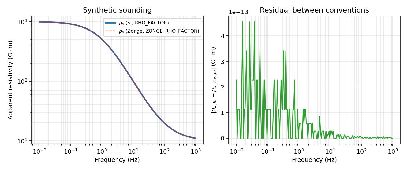
Left: the SI ((2)) and Zonge ((3)) curves sit on top of each other across five decades of frequency. Right: their difference stays below \(5\times10^{-13}\,\Omega\cdot\)m – floating-point noise, not a physical gap.

Because the two conventions are exact algebraic rearrangements of the same relation, this residual is expected to be at the limit of double-precision arithmetic everywhere, and it is. Note that pycsamt.core.base.MTBase keeps its own class-attribute copies of RHO_FACTOR, ZONGE_RHO_FACTOR, MU0/EPS0/C0/ETA0, computed with the same formulas – pycsamt.constants is the documented, importable canonical source, but not every consumer in the codebase has been switched over to importing it directly yet (pycsamt.zonge.z, pycsamt.zonge.proc_utils, and pycsamt.site.compute do import MU_0 from here).

2.3. Angles, Logarithms, And Tolerances

A smaller group of constants supports everyday numeric work rather than a specific physical law:

Name	Value	Use
PI	\(\pi\)	Base circular constant; also feeds DEG2RAD/RAD2DEG.
TAU	\(2\pi\)	Shorthand for angular-frequency conversions, \(\omega=\text{TAU}\times f\).
DEG2RAD / RAD2DEG	\(\pi/180\), \(180/\pi\)	Degree/radian conversion used across rotation and phase code.
LN10	\(\ln 10\)	Natural-log-of-ten factor for decade-based scaling (e.g. phase slope per Frequency decade).
MRAD	\(10^3\)	Radian-to-milliradian scale.
EPS_TOL	\(10^{-9}\)	Generic “close to zero” tolerance for float comparisons.
_RAD_THR / _DEG_SCALE	\(5^\circ\) in rad, \(180/\pi\)	Small-angle heuristics for auto-detecting whether a phase array is already in radians or degrees.

>>> from pycsamt.constants import PI, TAU, DEG2RAD, RAD2DEG, LN10, EPS_TOL
>>> PI, TAU
(3.141592653589793, 6.283185307179586)
>>> DEG2RAD, RAD2DEG
(0.017453292519943295, 57.29577951308232)
>>> LN10
2.302585092994046
>>> EPS_TOL
1e-09

_RAD_THR/_DEG_SCALE are exported from pycsamt.constants despite the leading underscore, but pycsamt.utils.zmath – the module that actually runs the degrees-vs-radians auto-detection – carries its own numerically identical pair rather than importing these, the same local-duplicate pattern seen with the apparent-resistivity factors above.

2.4. Unit Conversion Scales

A short list of plain multiplicative scales rounds out pycsamt.constants:

>>> from pycsamt.constants import (
...     MICROVOLTS_TO_VOLTS, PICOTESLA_TO_TESLA,
...     METERS_TO_KILOMETERS, PERCENT_FACTOR,
... )
>>> MICROVOLTS_TO_VOLTS, PICOTESLA_TO_TESLA
(1e-06, 1e-12)
>>> METERS_TO_KILOMETERS, PERCENT_FACTOR
(0.001, 100.0)

This set is narrower than what pycsamt.core.base.MTBase keeps locally – MTBase additionally defines NANOTESLA_TO_TESLA, MV_PER_KM_TO_V_PER_M, and Z_UNIT_MVK_NT_TO_SI for the mV/km-and-nT field-unit conversions used in the previous section’s worked example. If a new module needs those conversions, deriving them the same way (1e-9 and 1e-6 respectively, following the pattern of MICROVOLTS_TO_VOLTS/PICOTESLA_TO_TESLA already here) keeps the numbers traceable back to this one module.

2.5. Earth Radius And Geodesy Helpers

The Geodetic distance glossary entry gives the haversine formula pyCSAMT uses for nearest-station search:

(4)\[d = 2R \arcsin\!\left( \sqrt{\sin^2\tfrac{\Delta\phi}{2} + \cos\phi_1\cos\phi_2\sin^2\tfrac{\Delta\lambda}{2}} \right).\]

The radius \(R\) in (4) is pycsamt.constants._EARTH_R (a mean spherical Earth radius of 6,371,000 m), imported directly by pycsamt.site.location()’s pairwise-distance routine. A second, coarser helper, _M_PER_DEG (111,000 m per degree of latitude), is imported by pycsamt.site.profile to turn a small local patch of latitude/longitude into approximate along-profile metres without a full projection. Two other modules solve the same small-patch problem with their own, slightly different, locally defined constants instead of importing _M_PER_DEG – pycsamt.map.geometry splits it into separate _LON_M_PER_DEG/_LAT_M_PER_DEG (111,320 m / 110,574 m, reflecting that a degree of longitude shrinks with latitude while a degree of latitude does not), and pycsamt.models.occam2d.data shadows the same name with 111,195 m. None of these is wrong on its own – they are different spherical/ellipsoidal approximations chosen for different callers – but the three-way split is worth knowing about before assuming a metres-per-degree figure carries over unchanged between pyCSAMT subpackages.

2.6. UTM Zone Letters And Ellipsoids

pycsamt.gis.constants holds the lookup tables that pycsamt.gis.utils uses to convert geographic coordinates into UTM easting/northing. A UTM zone label combines a longitude-based zone number (not stored as a table – computed directly from longitude) with a latitude-based zone letter, which is a table lookup:

>>> from pycsamt.gis.constants import (
...     UTM_ZONE_DESIGNATOR, utm_letter_designator, ELLIPSOIDS, EPSG_PROJ4,
... )
>>> UTM_ZONE_DESIGNATOR["R"]
[24, 32]
>>> utm_letter_designator(25.77)
'R'
>>> wgs84 = next(e for e in ELLIPSOIDS if e[0] == 23)
>>> wgs84
[23, 'WGS-84', 6378137.0, 0.00669438]
>>> sorted(EPSG_PROJ4)[:3]
[3112, 4326, 28350]

Latitude \(25.77^\circ\) is the K2 Stratagem survey used throughout Coordinate Injection, which lands in band R (\(24^\circ\)N to \(32^\circ\)N). Twenty of the 21 entries in UTM_ZONE_DESIGNATOR are genuine disjoint 8-degree bands running from C at the south pole to X near the north pole; the 21st, Z, is a sentinel meaning “outside \(80^\circ\)S to \(84^\circ\)N” and spans the same range as every other band combined, so it has to be excluded when plotting the table as a set of non-overlapping bars:

import numpy as np
import matplotlib.pyplot as plt
from pycsamt.gis.constants import UTM_ZONE_DESIGNATOR, utm_letter_designator

bands = sorted(
    (kv for kv in UTM_ZONE_DESIGNATOR.items() if kv[0] != "Z"),
    key=lambda kv: kv[1][0],
)
fig, ax = plt.subplots(1, 1, figsize=(7.5, 3.2))
colors = plt.cm.turbo(np.linspace(0, 1, len(bands)))
for (letter, (lo, hi)), c in zip(bands, colors):
    ax.barh(0, hi - lo, left=lo, height=1.0, color=c, edgecolor="white")
    ax.text((lo + hi) / 2.0, 0, letter, ha="center", va="center", fontsize=9)

lat = 25.77
ax.axvline(lat, color="black", lw=1.2, ls="--")
ax.annotate(f"lat={lat}° -> {utm_letter_designator(lat)}",
            xy=(lat, 0.55), xytext=(lat, 0.85), ha="center", fontsize=8,
            arrowprops=dict(arrowstyle="-", lw=0.8))
ax.set(xlim=(-80, 84), ylim=(-0.6, 1.1), xlabel="Latitude (degrees)",
       title="UTM_ZONE_DESIGNATOR letter bands")
ax.set_yticks([])
fig.tight_layout()

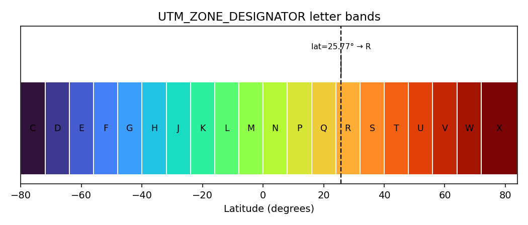
The 20 real UTM latitude bands, colour-coded, with the K2 survey’s \(25.77^\circ\)N marked – it falls inside band R, matching utm_letter_designator(25.77) above.

The Ellipsoid table works the same way: each row is [id, name, equatorial_radius_m, eccentricity_squared], and pycsamt.gis.utils.ll_to_utm() looks a row up by id before running the Bulletin-1532 projection equations. Passing WGS-84 (23) for the same K2 coordinates reproduces the easting/northing that Coordinate Injection reports for the injected station block:

>>> from pycsamt.gis.utils import ll_to_utm
>>> ll_to_utm(23, 25.77, 109.63)
('49R', 362619.51423243043, 2850927.3597707017)

EPSG_PROJ4 is a smaller, curated dictionary rather than a full EPSG registry – it maps a handful of EPSG codes actually exercised by pyCSAMT’s MARE2DEM and Australian-survey workflows to their Proj4 strings and zone numbers, not every code in the public EPSG dataset. Looking up a code outside that curated set (for example 32649, the WGS-84 UTM zone that the same K2 survey is reprojected into during coordinate injection) raises a plain KeyError rather than falling back to a computed projection, so callers needing an arbitrary EPSG code go through pycsamt.gis.utils’s pyproj-based path instead of this table.

2.7. Where Each Constant Is Consumed

Constant	Consumers
MU_0	pycsamt.zonge.z, pycsamt.zonge.proc_utils, pycsamt.zonge.avg, pycsamt.zonge.processing, pycsamt.site.compute, pycsamt.jones.j.
PI	Same pycsamt.zonge modules, for \(\omega=2\pi f\).
_EARTH_R	pycsamt.site.location (haversine Geodetic distance).
_M_PER_DEG	pycsamt.site.profile (local metric approximation).
RHO_FACTOR / ZONGE_RHO_FACTOR	Documented in pycsamt.core.base.MTBase; not currently imported from here by name, but numerically identical.
ELLIPSOIDS / utm_letter_designator / _EQUATORIAL_RADIUS_IDX / _ECC_SQUARED_IDX	pycsamt.gis.utils.ll_to_utm(), pycsamt.gis.utils.utm_to_ll().
UTM_ZONE_DESIGNATOR	pycsamt.gis.utils zone-letter lookup; pycsamt.property keeps an independent copy of the same table.

Reading the modules through this lens explains why two pages in this documentation can quote the same-looking number (\(0.2\), or \(6{,}371{,}000\) m) without one importing the other: they are independently derived from the same handful of constants rather than copy-pasted, and this page is where that shared origin is made explicit. Continue to Impedance Tensor for how RHO_FACTOR fits into the full tensor formulation, or to Coordinate Injection for the K2 UTM/Gauss-Kruger reconciliation referenced above.