
9. Maxwell Forward Modelling and Solver Contracts#
Electromagnetic inversion is meaningful only through the forward problem that
connects an earth model to observable fields. The
pycsamt.forward.maxwell package is the boundary where pyCSAMT makes that
connection explicit. It does not present every numerical solver as equivalent.
It defines immutable mesh, problem, receiver, result, diagnostic, capability,
benchmark, cache, and batch contracts; a numerical backend enters this namespace
only through an adapter that declares and enforces what it can actually solve.
That distinction matters in routine work. A conductivity array is not yet a Maxwell problem. It needs a coordinate system, cell geometry, air and earth regions, frequencies, receiver locations, tensor components, time convention, boundary treatment, and an identified solver. Likewise, a complex response array is not yet scientific evidence. Its axes must match the problem exactly, and its convergence and validity diagnostics must pass a declared policy.
This page develops the physics and numerical reasoning behind those contracts, then shows how to construct and assess them with the public API. The practical AI workflow in Solver-neutral Maxwell contracts builds on the same foundation.
9.1. From Maxwell’s equations to an MT response#
For harmonic fields with the time dependence \(\exp(+i\omega t)\), Maxwell’s equations in an isotropic conductive earth can be written
where \(\mathbf E\) is electric field, \(\mathbf H\) magnetic field, \(\mathbf J_s\) an imposed source current, \(\sigma\) conductivity, \(\varepsilon\) permittivity, and \(\mu\) permeability. In the magnetotelluric frequency range and a sufficiently conductive earth, displacement current is commonly neglected when
Eliminating \(\mathbf H\) then gives a curl–curl equation,
Signs change consistently under \(\exp(-i\omega t)\). This is why
MaxwellProblem.time_dependence is a physical input and why a backend must
declare supported conventions. Mixing conventions conjugates phase behavior;
it cannot be repaired by relabeling a plot.
At a surface receiver, the horizontal impedance tensor relates electric and magnetic fields,
The canonical component names in pyCSAMT are zxx, zxy, zyx, and
zyy. A 2-D earth invariant along one horizontal direction separates into
TE and TM modes and supports the off-diagonal components zxy and zyx.
Asking a 2-D problem for diagonal components is therefore rejected by the
contract rather than filled with arbitrary zeros.
Apparent resistivity and phase are derived responses,
The solver contract retains complex impedance because its real and imaginary parts preserve the quantity directly returned by the field ratio. Derived features can always be calculated later with the same unit and sign convention.
9.2. Why diffusion controls the mesh scale#
In a uniform conductor, equations (1) and (2) lead to a complex propagation constant. The amplitude decay scale is the skin depth
For \(\mu=\mu_0\), this is approximately
>>> from pycsamt.forward.maxwell import skin_depth_m
>>> round(float(skin_depth_m(100, 1)))
5033
>>> round(float(skin_depth_m(10, 1000)))
50
The smallest skin depth usually comes from the most conductive material at the highest frequency. It sets a demanding local cell scale. The largest skin depth, often associated with low frequency and resistive material, motivates the extent of the earth and padding. These two requirements compete: a mesh that is fine enough everywhere and wide enough everywhere can become enormous, especially in 3-D.
Skin depth is only a planning scale. Thin layers, sharp contacts, receiver interpolation, topography, anisotropy, and discretization error can require finer cells. Conversely, padding far from receivers may grow because it mainly moves an artificial boundary away from the sensitive region.
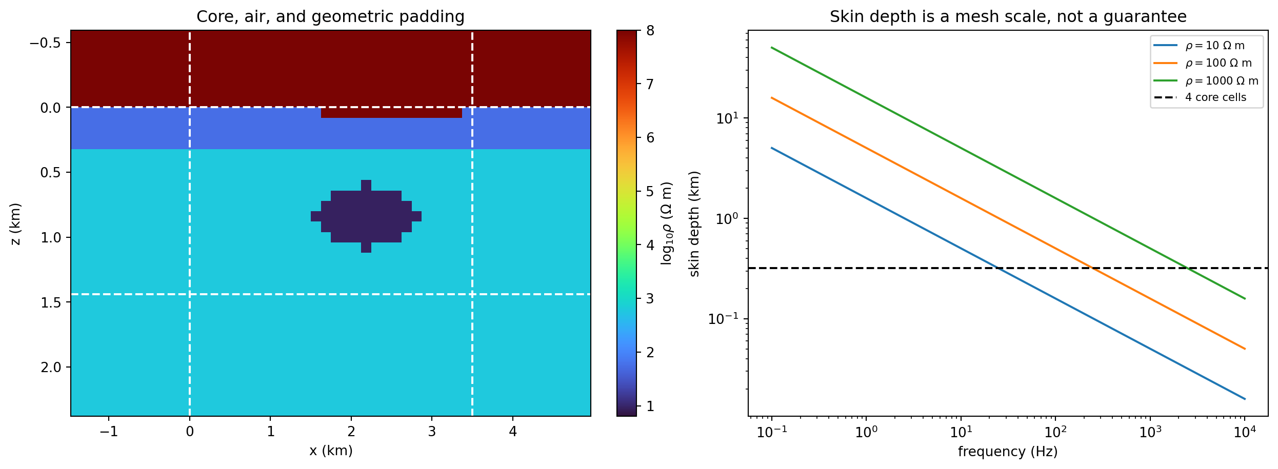
The left panel separates the geological core with dashed lines from air,
horizontal padding, and bottom padding. Padding conductivity is extended from
the nearest earth cells, while the terrain mask replaces cells above the local
surface with numerical air. The right panel shows that frequency and
resistivity jointly control penetration. Its horizontal line is only a
four-cell scale. In the executed example the minimum skin depth contains
0.38 core cells, so the mesh is deliberately too coarse for the most
conductive, highest-frequency case. The warning is actionable numerical
evidence, not an exception to hide.
9.3. The canonical mesh contract#
MaxwellMesh stores strictly increasing cell
edges, not only an image shape. Its canonical array order is (z, x) in 2-D
and (z, y, x) in 3-D. Depth increases downward. Horizontal coordinates
and the optional CRS remain attached to the mesh.
>>> from pycsamt.forward.maxwell import MaxwellMesh
>>> mesh = MaxwellMesh(
...     x_edges_m=[0, 100, 250, 500],
...     z_edges_m=[0, 50, 150, 350],
...     crs="EPSG:32630",
... )
>>> mesh.dimension, mesh.shape
(2, (3, 3))
>>> mesh.cell_widths_m["x"].tolist()
[100.0, 150.0, 250.0]
>>> mesh.cell_centres_m["z"].tolist()
[25.0, 100.0, 250.0]
Edges make cell width, volume, adjacency ratio, receiver containment, and
interpolation unambiguous. A tuple such as (30, 40) cannot reveal whether
cells are 10 m or 10 km wide, uniform or geometrically stretched.
The arrays returned by the contracts are read-only. This prevents a problem hash from referring to one model while an in-place mutation silently changes the conductivity later. To alter a physical input, create a new contract and therefore a new hash.
9.4. Building a solver mesh from geology#
The geological grid describes the region where the earth model is interpreted.
A solver mesh normally needs more: air layers, horizontal padding, bottom
padding, extended material values, and explicit region masks.
build_solver_mesh() performs that transformation
without choosing a numerical backend.
>>> import numpy as np
>>> from pycsamt.ai.geology import GeologyGrid
>>> from pycsamt.forward.maxwell import MeshDesign, build_solver_mesh
>>> grid = GeologyGrid.regular_2d(
...     nx=20, nz=12, dx_m=150, dz_m=100,
... )
>>> rho = np.full(grid.shape, 300.0)
>>> rho[:3] = 40.0
>>> design = MeshDesign(
...     horizontal_padding_cells=(4, 4),
...     bottom_padding_cells=5,
...     air_layers=4,
...     padding_expansion=1.3,
...     air_expansion=1.2,
... )
>>> solver_model = build_solver_mesh(
...     grid,
...     resistivity_ohm_m=rho,
...     frequencies_hz=[100, 10, 1],
...     design=design,
... )
>>> solver_model.mesh.shape
(21, 28)
>>> solver_model.core_slices
(slice(4, 16, None), slice(4, 24, None))
>>> solver_model.quality.cell_count
588
Exactly one of conductivity_s_m and resistivity_ohm_m must be supplied.
The returned model always stores conductivity in SI units. This explicit
conversion avoids a particularly destructive error: passing resistivity values
to a solver that expects conductivity.
The core slices map the original geological model into the padded array. They are essential when a response-based optimization runs on the solver mesh but the recovered model must be exported on the geological grid. Do not reconstruct them from padding counts after serialization; use the stored contract.
9.4.1. What MeshDesign controls#
horizontal_padding_cells accepts a symmetric integer or a low/high pair.
bottom_padding_cells extends the deepest model value. air_layers adds
cells above depth zero. padding_expansion and air_expansion are
geometric growth factors moving away from the core.
For core boundary cell width \(h_0\) and growth factor \(g\), padding width \(k\) is
and the total extent of \(n\) cells is
Large growth moves the boundary away with few cells but creates abrupt width changes. Small growth is smoother but increases cell count. The correct choice is established by mesh convergence, not appearance.
air_conductivity_s_m is a positive numerical conductivity, not geological
resistivity. Zero conductivity can make discrete systems singular or violate
backend assumptions. Whether air should also be marked inactive depends on
the backend capability.
9.4.2. Topography is a physical region mask#
An aligned TopographicSurface defines the local
depth of earth. The builder interpolates that surface onto padded horizontal
cell centres and constructs complementary earth_mask and air_mask
arrays. It does not merely warp a display.
>>> from pycsamt.ai.geology import TopographicSurface
>>> elevation = 420 + 25 * np.sin(
...     2 * np.pi * grid.x_m / np.ptp(grid.x_m)
... )
>>> surface = TopographicSurface(
...     grid, elevation, float(elevation.max()),
...     source="station elevations",
... )
>>> topo_model = build_solver_mesh(
...     grid, resistivity_ohm_m=rho,
...     frequencies_hz=[100, 10, 1],
...     topography=surface, design=design,
... )
>>> topo_model.earth_mask.shape == topo_model.mesh.shape
True
>>> np.array_equal(topo_model.air_mask, ~topo_model.earth_mask)
True
Topography and the grid must share dimension, coordinates, and CRS. Failing early is preferable to aligning two arrays by shape when they represent different locations.
9.4.3. Reading mesh-quality diagnostics#
MeshQuality records total cells, width
extremes, global aspect ratio, worst adjacent-width ratio, minimum skin depth,
cells per minimum skin depth, and advisory warnings. Its acceptable
property means only that configured advisory limits were not violated. It is
not proof of forward accuracy.
The reported global width ratio is
while the adjacent ratio is
The first describes overall scale separation; the second detects abrupt local growth. A large global ratio can be acceptable across many gradual padding cells, whereas a large adjacent ratio can damage numerical accuracy locally.
If the skin-depth warning fires, possible corrections are to refine core cells,
remove unreliable high frequencies, limit unrealistically conductive prior
values, or use local refinement supported by another mesh builder/backend. Do
not simply lower minimum_cells_per_skin_depth to make the warning disappear.
9.5. The solver-neutral Maxwell problem#
MaxwellProblem binds the complete physical
input. Its required relationships are validated at construction:
conductivity is positive, finite, and shaped like the mesh;
receiver dimension equals mesh dimension;
frequencies are positive, finite, and unique;
component names are canonical and unique;
2-D components are restricted to
zxyandzyx;active cells match the mesh and include at least one cell;
permeability is positive and the time convention is supported by the contract;
metadata is finite and JSON-compatible.
Receivers are a separate contract because names, coordinates, and orientation are part of output identity.
>>> from pycsamt.forward.maxwell import ReceiverSet
>>> receivers = ReceiverSet(
...     [[450, 0], [1050, 0], [1650, 0], [2250, 0]],
...     ["S01", "S02", "S03", "S04"],
... )
>>> topo_model.assess_receivers(receivers)
()
>>> problem = topo_model.to_problem(
...     [100, 10, 1], receivers,
...     components=("zxy", "zyx"),
...     mark_air_inactive=False,
...     metadata={"survey": "teaching-line"},
... )
>>> problem.mesh.dimension, problem.receivers.count
(2, 4)
>>> len(problem.problem_hash)
64
assess_receivers reports positions outside the mesh or below the local
discretized terrain without silently snapping them. The example retains air
as active low-conductivity cells because the in-repository mt2d adapter does
not support inactive cells or topographic masks. That also means a truly
topographic problem is not within that adapter’s stated capability merely
because a padded conductivity array can be formed.
9.5.1. Problem hashes and provenance#
The deterministic SHA-256 problem_hash covers conductivity, frequencies,
active cells, mesh, receivers, components, convention, permeability, and
metadata. It is the identity used to validate results and key caches.
A changed station order produces a changed problem even if coordinates are the same, because output axis order changes. A changed metadata field also changes the hash by design; metadata should therefore contain stable physical provenance, not timestamps that differ on every identical run.
9.6. Backend capabilities are scientific claims#
BackendCapabilities declares dimension,
components, time conventions, nonuniform-mesh support, inactive-cell support,
topography, anisotropy, cell/frequency limits, and verified benchmarks.
>>> from pycsamt.forward.maxwell import BackendCapabilities
>>> capability = BackendCapabilities(
...     name="teaching-backend", version="1.0",
...     dimensions=(2,), components=("zxy", "zyx"),
...     supports_nonuniform_mesh=True,
...     supports_inactive_cells=False,
...     supports_topography=False,
...     maximum_cells=10000,
...     verified_benchmarks=("half-space",),
... )
>>> report = capability.assess(problem)
>>> report.compatible
True
>>> report.errors
()
A capability declaration does not certify itself. verified_benchmarks
must correspond to stored outcomes for the exact adapter and solver version.
Changing translation logic or numerical dependencies can require the adapter
version and evidence to be updated together.
Compatibility assessment is preflight, not execution. It gathers hard errors such as wrong dimension, unsupported components, inactive cells, nonuniform mesh, topography, or size limits before an expensive solve begins. Warnings are advisory validation concerns. Users can inspect both; adapters call the same assessment automatically.
9.7. The adapter lifecycle#
An adapter translates between the canonical contracts and one backend’s native input/output. It is deliberately more than a thin wrapper.
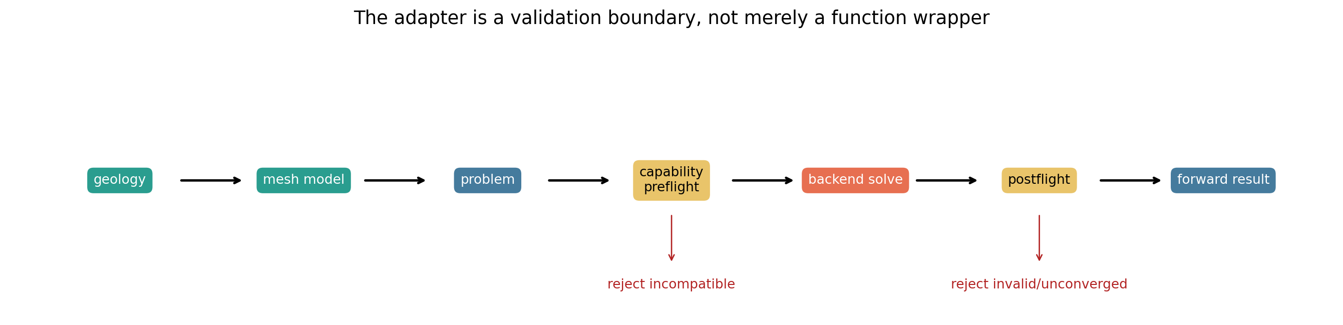
Preflight rejects problems outside declared capabilities. The backend then solves only compatible input. Postflight verifies result type, problem hash, frequency order, station order, components, backend identity, convergence, residual threshold, and response validity. A backend cannot silently return a smaller frequency set or reordered stations and still pass.
AdapterPolicy controls result acceptance:
>>> from pycsamt.forward.maxwell import AdapterPolicy
>>> policy = AdapterPolicy(
...     require_convergence=True,
...     maximum_relative_residual=1e-6,
...     require_all_valid=True,
... )
>>> policy.maximum_relative_residual
1e-06
The exceptions distinguish failure stages:
IncompatibleProblemErrormeans preflight rejected the physics or numerical scope;BackendExecutionErrorwraps an ordinary solver failure;InvalidBackendResultErrormeans output violated the canonical contract;SolverConvergenceErrormeans diagnostics or validity failed policy.
Treating all four as a generic empty result would destroy the evidence needed to correct the workflow.
9.7.1. Adapting a trusted callable#
CallableMaxwellAdapter is useful when a
trusted Python callable already accepts MaxwellProblem and returns a fully
formed ForwardResult. It does not convert arbitrary arrays automatically;
the callback remains responsible for canonical output and diagnostics.
>>> from pycsamt.forward.maxwell import (
...     BackendCapabilities, CallableMaxwellAdapter,
...     ForwardResult, SolverDiagnostics, half_space_impedance,
... )
>>> demo_capability = BackendCapabilities(
...     "analytic-demo", "1", (2,), ("zxy", "zyx"),
... )
>>> def analytic_solver(value):
...     z = np.zeros((value.receivers.count,
...                   len(value.frequencies_hz),
...                   len(value.components)), dtype=complex)
...     reference = half_space_impedance(
...         100.0, value.frequencies_hz,
...     )
...     z[:] = reference[None, :, None]
...     diagnostics = SolverDiagnostics(
...         np.ones((len(value.frequencies_hz), 1), bool),
...         np.zeros((len(value.frequencies_hz), 1), int),
...         np.zeros((len(value.frequencies_hz), 1)), 0.0,
...     )
...     return ForwardResult(
...         value.problem_hash, value.frequencies_hz,
...         value.receivers.names, value.components,
...         z, None, "analytic-demo", "1", diagnostics,
...     )
>>> adapter = CallableMaxwellAdapter(
...     demo_capability, analytic_solver, policy,
... )
>>> result = adapter.solve(problem)
>>> result.shape, result.success
((4, 3, 2), True)
This example is an analytic half-space response used to demonstrate the
contract. It is not a multidimensional solution of the heterogeneous
problem conductivity. Naming it analytic-demo prevents that distinction
from being hidden behind a plausible response array.
9.8. In-repository and external adapters#
MT2DAdapter translates compatible problems to the in-repository 2-D
finite-difference implementation. Its declared scope is precise:
two-dimensional
zxyandzyxresponses;surface receivers at
z=0;\(\exp(+i\omega t)\);
vacuum permeability;
nonuniform meshes;
no inactive cells, topography, or anisotropy.
It declares passing half-space and layered-earth benchmarks. These statements are stronger and more useful than saying merely that “2-D is supported.”
MT3DAdapter is explicitly research-only. It supports uniform 3-D meshes
and all four impedance components but defaults to a 6,000-cell safety ceiling,
has no inactive cells or topography, and is not a production-scale 3-D solver.
Increasing the ceiling changes computational risk, not numerical maturity.
ModEm3DAdapter provides an external-process integration. External adapters
must additionally resolve an executable, isolate a run directory, write native
files, execute under a timeout policy, parse output, convert units, and retain
stdout/stderr provenance. Availability of an executable is not the same as
compatibility of a problem or validation of its result.
The external run policy controls timeout, environment, retained workspaces, and process behavior. A reproducible record should preserve executable path and version, command arguments, native input hashes, return code, and parsed-output identity. Never infer success solely because a results file exists; it may be stale or incomplete.
9.9. Lazy backend registration#
The registry stores factories rather than importing every optional solver when
pycsamt.forward.maxwell is imported. This keeps the core contracts usable
without external executables or optional solver libraries.
>>> from pycsamt.forward.maxwell import (
...     create_backend, list_backends, register_mt2d_backend,
... )
>>> register_mt2d_backend(replace=True)
>>> "mt2d" in list_backends()
True
>>> mt2d = create_backend("mt2d", verbose=False)
>>> mt2d.capabilities.dimensions
(2,)
>>> mt2d.capabilities.verified_benchmarks
('half-space', 'layered-earth')
Registration is process-wide. replace=True should be explicit because
silently replacing a factory could change numerical behavior elsewhere in a
long-running experiment. List capability metadata before creating or running
a backend when building user-facing selection interfaces.
9.10. Canonical results and diagnostics#
ForwardResult stores impedance with shape
(station, frequency, component). It includes all three axis labels, a
validity mask, backend identity, problem hash, diagnostics, and metadata.
SolverDiagnostics records convergence,
iterations, and relative residual for each frequency/source solve plus total
runtime. For a linear system
a common reported relative residual is
A small algebraic residual says the discrete system was solved accurately. It does not prove that the mesh, boundary condition, source representation, or earth model accurately represents the continuous problem. Solver convergence and mesh convergence answer different questions.
>>> result.backend_name, result.backend_version
('analytic-demo', '1')
>>> result.receiver_names
('S01', 'S02', 'S03', 'S04')
>>> result.components
('zxy', 'zyx')
>>> result.diagnostics.success
True
>>> result.validate_against(problem) is None
True
The validity mask separates missing or unusable responses from legitimate complex zeros. Downstream misfit code should combine it with observed-data validity rather than replacing invalid entries by zero.
9.11. Analytic benchmarks before geological complexity#
A half-space has a closed-form impedance under the package convention,
with the square-root branch consistent with the chosen time dependence. Its apparent resistivity is constant and its phase is 45 degrees in the ideal quasi-static case. A layered-earth recurrence provides a stronger frequency- dependent reference.
>>> from pycsamt.forward.maxwell import (
...     half_space_impedance, layered_earth_impedance,
... )
>>> frequencies = np.array([100.0, 10.0, 1.0])
>>> z_half = half_space_impedance(100.0, frequencies)
>>> np.round(np.rad2deg(np.angle(z_half)), 1).tolist()
[45.0, 45.0, 45.0]
>>> z_layered = layered_earth_impedance(
...     [30.0, 600.0, 10.0], [250.0, 700.0], frequencies,
... )
>>> z_layered.shape
(3,)
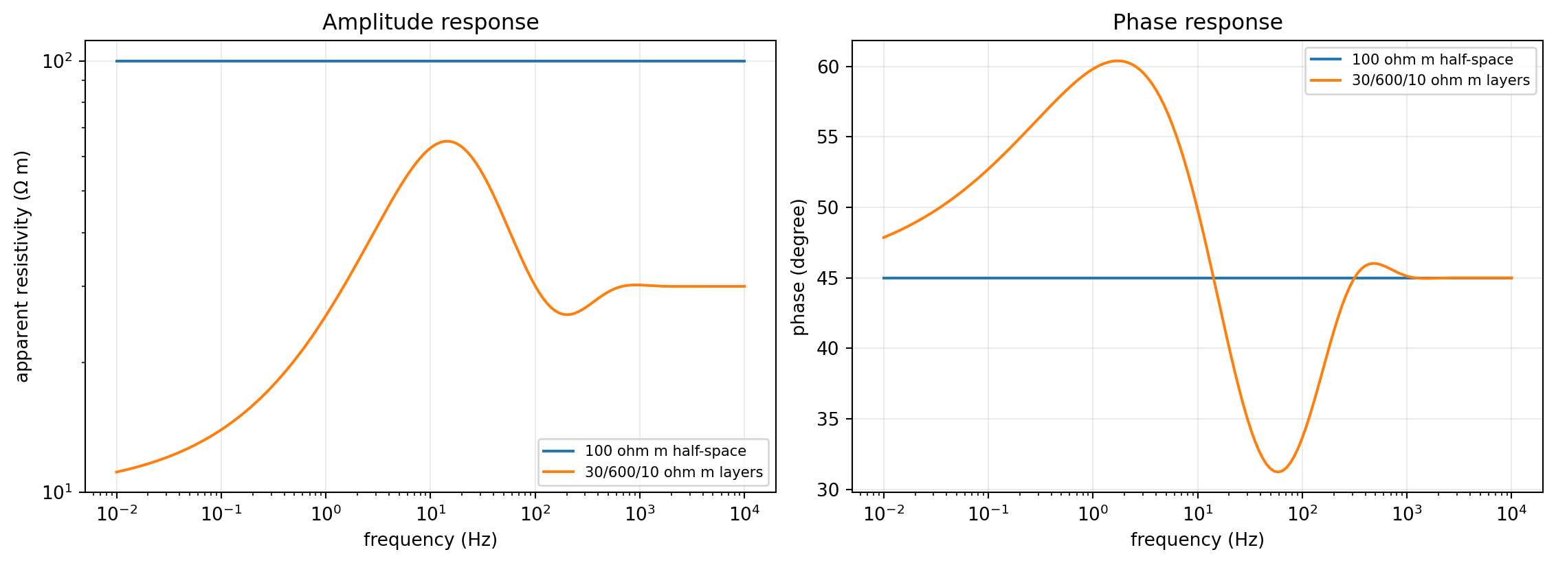
The half-space curve remains flat in apparent resistivity and constant in phase. The layered model changes with frequency because the relative influence of its conductive cover, resistive middle layer, and conductive basement changes with penetration. A solver that cannot reproduce these responses within declared amplitude and phase tolerances should not be trusted on a more complicated geology merely because its image looks smooth.
9.11.1. Executable benchmark objects#
half_space_benchmark and layered_earth_benchmark package a problem,
analytic reference, and identity. run_benchmarks evaluates an adapter and
returns metrics against BenchmarkThresholds.
The default criteria include normalized complex RMS, maximum relative amplitude
error, maximum phase error, valid fraction, and convergence.
For prediction \(Z_j\) and reference \(Z_j^*\), normalized RMS is
Circular phase error must wrap differences into a principal interval so values near \(-180^\circ\) and \(180^\circ\) are recognized as neighbors. Amplitude, phase, validity, and convergence gates are retained separately; passing one cannot compensate for failing another.
9.12. Mesh-convergence evidence#
Analytic agreement on canonical cases is necessary but not sufficient. For a representative model, solve a sequence of meshes with characteristic core sizes \(h\), \(h/r\), and \(h/r^2\). Compare responses after exact axis alignment. A relative change measure is
The result is credible only when changes decline toward the application tolerance and the finest mesh is itself within capability limits. Perform similar tests for padding extent and boundary placement. A single fine-looking mesh supplies no convergence trend.
Topography convergence should refine both horizontal terrain sampling and vertical cells near the surface. If moving receivers between terrain and a flat reference changes the physical question, do not mix that geometry change with mesh refinement in the same comparison.
9.13. Caching without confusing identity#
MaxwellResultCache stores results under stable
keys with file digests and locking. A cache hit is valid only when the exact
problem and expected backend identity match. Cache statistics distinguish hits,
misses, writes, and corrupt entries.
Caching is especially valuable for AI dataset generation and repeated loss evaluation because Maxwell solves dominate cost. It must not conceal a solver upgrade: include backend version in the cache expectation or use a new cache namespace. Corruption errors should trigger quarantine or recomputation, never silent acceptance of a partially written archive.
Concurrent writers require locking. A lock timeout means another process may be producing the same key or a stale lock needs investigation. Deleting broad cache directories automatically is not an appropriate response; preserve the failure and resolve the exact entry.
9.14. Batch solving and failure manifests#
solve_batch applies one adapter to multiple problems with a
BatchPolicy. Batch behavior must distinguish
fail-fast scientific experiments from large synthetic campaigns where a small
number of documented failures can be retained and retried.
A FailureManifest stores the problem hash,
failure type, message, and position. This is essential because dropping failed
realizations without recording why can bias a training distribution. For
example, if high-contrast conductive bodies fail more often, silently removing
them narrows the prior and makes the eventual inverse model weakest on the very
targets of interest.
Batch parallelism should respect backend thread safety, external executable licenses, memory per solve, and cache locking. More workers can reduce throughput when sparse factorizations compete for memory. Benchmark sustained throughput and failure rate, not only the fastest individual solve.
9.15. Choosing a backend responsibly#
Backend selection begins with the physical question:
Is the earth approximation 1-D, 2-D, or genuinely 3-D?
Which impedance components and time convention are required?
Are cells nonuniform, inactive, anisotropic, or topographic?
Are receivers on the surface or buried?
How many cells and frequencies does the problem require?
Which canonical benchmarks has the exact version passed?
What mesh-convergence evidence exists at comparable contrasts and geometry?
Only after those questions should runtime and convenience decide among compatible backends. A fast solver outside its declared dimension or terrain support is not an approximation with known error; it is a different problem.
9.16. Common failure modes#
The mesh builds but quality is unacceptable. The builder validates data structure and reports advisory numerical risks. Refine the core, adjust the frequency band, examine extreme conductivity, or redesign padding. Do not equate successful construction with adequate discretization.
A topographic model is rejected by ``mt2d``. The mesh builder can represent topographic air/earth regions, but the adapter does not claim inactive-cell or topography support. Use a validated capable backend or explicitly solve a flat- surface approximation and state that limitation.
Receivers are below local terrain. Check the vertical datum, the meaning of
depth zero, station/topography alignment, and coordinate order. Automatic
snapping would conceal these errors, so assess_receivers reports them.
The solver converges but benchmarks fail. Algebraic convergence applies to the implemented discrete system. Investigate field normalization, boundary conditions, sign convention, receiver interpolation, units, and mesh extent.
The result has the right shape but validation fails. A reordered frequency,
station, or component axis is scientifically different despite equal shape.
Return the axes exactly as supplied by MaxwellProblem.
A 3-D solve exceeds the cell ceiling. The research adapter’s direct sparse method is not production-scalable. Coarsening until it runs may destroy the physics. Prefer a validated external production backend and establish mesh convergence within available resources.
Responses look identical across heterogeneous models. Confirm conductivity
was not passed as resistivity, the model was mapped into core_slices, the
backend actually consumes the supplied array, and cached results use different
problem hashes.
Phase has the opposite sign. Check time dependence, impedance definition, component orientation, and unit conversion before applying any manual sign change. The convention must be consistent through analytic reference, backend, observations, and plots.
9.17. What reproducibility requires#
A defensible forward result should retain:
geological model coordinates, units, CRS, and property parameterization;
the complete
MeshDesign, solver mesh edges, core slices, region masks, model hash, and quality warnings;receiver names, coordinates, orientation, and topography/datum source;
frequencies, components, time convention, permeability, and problem hash;
backend and adapter name/version, executable version where applicable, and capability report;
boundary conditions and native solver settings not represented by the common contract;
convergence, iterations, residuals, validity, runtime, and backend messages;
benchmark outcomes and mesh-convergence evidence for the declared use;
cache identity or external run-directory provenance when used.
The provenance(), to_dict(), and archive methods on the contracts provide
the machine-readable foundation. They do not replace the scientific narrative
explaining why the mesh and backend are suitable.
9.18. Relationship to inversion and AI datasets#
In classical inversion, the forward operator is evaluated repeatedly as the earth model changes. Numerical error must remain below the data-error scale; otherwise the optimizer can fit discretization artifacts. Mesh and solver identity should remain fixed during one objective comparison unless the change is explicitly accounted for.
In supervised AI inversion, each label-response pair is
where \(h\) denotes mesh/discretization and \(b\) backend. A network can learn systematic error in \(\mathcal F_{h,b}\) as readily as earth physics. Dataset manifests must therefore retain problem hashes, backend versions, diagnostics, and failures. Cross-solver validation on a subset estimates how strongly the learned distribution depends on one implementation.
For response-consistency losses, predictions must be mapped from the geological grid to the same solver mesh and evaluated through a compatible adapter. A skin-depth proxy or analytic half-space response is useful for teaching and unit tests but is not a substitute for heterogeneous Maxwell evidence.
9.19. Reproduce the figures#
View and copy the complete Maxwell theory figure generatorClick to inspect and copy the complete code
  1#!/usr/bin/env python
  2# Author: LKouadio <etanoyau@gmail.com>
  3# License: LGPL-3.0
  4"""Generate executed figures for theory/maxwell_forward.rst."""
  5
  6from __future__ import annotations
  7
  8import sys
  9from pathlib import Path
 10
 11import matplotlib
 12
 13matplotlib.use("Agg")
 14import matplotlib.pyplot as plt
 15import numpy as np
 16
 17ROOT = Path(__file__).resolve().parents[2]
 18sys.path.insert(0, str(ROOT))
 19
 20from pycsamt.ai.geology import GeologyGrid, TopographicSurface  # noqa: E402
 21from pycsamt.forward.maxwell import (  # noqa: E402
 22    MeshDesign,
 23    build_solver_mesh,
 24    half_space_impedance,
 25    layered_earth_impedance,
 26    skin_depth_m,
 27)
 28
 29IMAGE_DIR = ROOT / "docs/source/images/theory"
 30
 31
 32def _save(fig: plt.Figure, name: str) -> None:
 33    IMAGE_DIR.mkdir(parents=True, exist_ok=True)
 34    fig.savefig(IMAGE_DIR / name, dpi=190, bbox_inches="tight")
 35    plt.close(fig)
 36
 37
 38def make_mesh_anatomy() -> tuple[int, float, int]:
 39    grid = GeologyGrid.regular_2d(nx=28, nz=18, dx_m=125, dz_m=80)
 40    z, x = np.mgrid[:18, :28]
 41    rho = np.full(grid.shape, 600.0)
 42    rho[z < 4] = 55.0
 43    rho[((x - 17) / 5) ** 2 + ((z - 10) / 3) ** 2 <= 1] = 9.0
 44    elevation = 440 + 42 * np.sin(2 * np.pi * grid.x_m / np.ptp(grid.x_m))
 45    topo = TopographicSurface(grid, elevation, float(elevation.max()), source="synthetic")
 46    model = build_solver_mesh(
 47        grid,
 48        resistivity_ohm_m=rho,
 49        frequencies_hz=np.geomspace(.5, 1000, 14),
 50        topography=topo,
 51        design=MeshDesign(horizontal_padding_cells=5, bottom_padding_cells=5,
 52                          air_layers=5, padding_expansion=1.3, air_expansion=1.2),
 53    )
 54    display = np.log10(1 / model.conductivity_s_m)
 55    xe, ze = model.mesh.x_edges_m / 1000, model.mesh.z_edges_m / 1000
 56    fig, axes = plt.subplots(1, 2, figsize=(13, 4.7), constrained_layout=True)
 57    im = axes[0].pcolormesh(xe, ze, display, cmap="turbo", shading="flat", vmin=.8, vmax=8)
 58    cs = model.core_slices
 59    axes[0].axvline(model.mesh.x_edges_m[cs[1].start] / 1000, color="white", ls="--")
 60    axes[0].axvline(model.mesh.x_edges_m[cs[1].stop] / 1000, color="white", ls="--")
 61    axes[0].axhline(model.mesh.z_edges_m[cs[0].start] / 1000, color="white", ls="--")
 62    axes[0].axhline(model.mesh.z_edges_m[cs[0].stop] / 1000, color="white", ls="--")
 63    axes[0].invert_yaxis(); axes[0].set(title="Core, air, and geometric padding", xlabel="x (km)", ylabel="z (km)")
 64    fig.colorbar(im, ax=axes[0], label=r"$\log_{10}\rho$ ($\Omega$ m)")
 65    frequencies = np.geomspace(.1, 10000, 200)
 66    for value in (10, 100, 1000):
 67        axes[1].loglog(frequencies, skin_depth_m(value, frequencies) / 1000,
 68                       label=fr"$\rho={value}\ \Omega$ m")
 69    axes[1].axhline(.08 * 4, color="black", ls="--", label="4 core cells")
 70    axes[1].set(title="Skin depth is a mesh scale, not a guarantee", xlabel="frequency (Hz)", ylabel="skin depth (km)")
 71    axes[1].legend(fontsize=8)
 72    _save(fig, "maxwell_mesh_anatomy.png")
 73    return model.quality.cell_count, model.quality.cells_per_minimum_skin_depth, len(model.quality.warnings)
 74
 75
 76def make_analytic_responses() -> tuple[float, float]:
 77    f = np.geomspace(.01, 10000, 160)
 78    half = half_space_impedance(100, f)
 79    layered = layered_earth_impedance([30, 600, 10], [250, 700], f)
 80    mu0 = 4e-7 * np.pi
 81    fig, axes = plt.subplots(1, 2, figsize=(11.8, 4.2), constrained_layout=True)
 82    for values, label in ((half, "100 ohm m half-space"), (layered, "30/600/10 ohm m layers")):
 83        rhoa = np.abs(values) ** 2 / (mu0 * 2 * np.pi * f)
 84        phase = np.rad2deg(np.angle(values))
 85        axes[0].loglog(f, rhoa, label=label)
 86        axes[1].semilogx(f, phase, label=label)
 87    axes[0].set(title="Amplitude response", xlabel="frequency (Hz)", ylabel=r"apparent resistivity ($\Omega$ m)")
 88    axes[1].set(title="Phase response", xlabel="frequency (Hz)", ylabel="phase (degree)")
 89    for ax in axes: ax.legend(fontsize=8); ax.grid(alpha=.25)
 90    _save(fig, "maxwell_analytic_benchmarks.png")
 91    return float(np.min(np.abs(layered))), float(np.max(np.abs(layered)))
 92
 93
 94def make_adapter_lifecycle() -> None:
 95    labels = ["geology", "mesh model", "problem", "capability\npreflight",
 96              "backend solve", "postflight", "forward result"]
 97    colors = ["#2a9d8f", "#2a9d8f", "#457b9d", "#e9c46a", "#e76f51", "#e9c46a", "#457b9d"]
 98    fig, ax = plt.subplots(figsize=(14, 3.3), constrained_layout=True)
 99    ax.set_xlim(-.6, 6.6); ax.set_ylim(-1.0, 1.1); ax.axis("off")
100    for i, (label, color) in enumerate(zip(labels, colors)):
101        ax.text(i, 0, label, ha="center", va="center", fontsize=10,
102                bbox=dict(boxstyle="round,pad=.55", fc=color, ec="white", lw=1.5), color="white" if color != "#e9c46a" else "black")
103        if i < len(labels) - 1:
104            ax.annotate("", (i + .68, 0), (i + .32, 0), arrowprops=dict(arrowstyle="->", lw=1.8))
105    ax.annotate("", (3, -.62), (3, -.24),
106                arrowprops=dict(arrowstyle="->", color="#b22222"))
107    ax.text(3, -.8, "reject incompatible", ha="center", color="#b22222")
108    ax.annotate("", (5, -.62), (5, -.24),
109                arrowprops=dict(arrowstyle="->", color="#b22222"))
110    ax.text(5, -.8, "reject invalid/unconverged", ha="center", color="#b22222")
111    ax.set_title("The adapter is a validation boundary, not merely a function wrapper", fontsize=14)
112    _save(fig, "maxwell_adapter_lifecycle.png")
113
114
115def main() -> int:
116    cells, cps, warnings = make_mesh_anatomy()
117    zmin, zmax = make_analytic_responses()
118    make_adapter_lifecycle()
119    print("solver mesh cells:", cells)
120    print("cells per minimum skin depth:", f"{cps:.2f}")
121    print("mesh quality warnings:", warnings)
122    print("layered impedance magnitude range:", f"{zmin:.6g}", f"{zmax:.6g}")
123    print("figures generated: 3")
124    return 0
125
126
127if __name__ == "__main__":
128    raise SystemExit(main())
Executed output:
solver mesh cells: 1064
cells per minimum skin depth: 0.38
mesh quality warnings: 1
layered impedance magnitude range: 0.000937496 1.53906
figures generated: 3
Continue with Impedance Tensor for tensor interpretation, Dimensionality, Distortion, And The Phase Tensor for selecting an earth approximation, Inversion Concepts for the inverse objective, and Foundations of AI Inversion for the role of Maxwell simulations in learned inversion.