
7. Dimensionality, Distortion, And The Phase Tensor#
Impedance Tensor introduces the phase tensor as a real, distortion- resistant object built from \(\mathbf{Z}\), and CSAMT, AMT, and MT Overview and Inversion Concepts both lean on Dimensionality as a modelling choice without saying exactly how it is measured. This page closes that gap: it derives the phase tensor’s orientation and skew angles, uses them to classify 1-D/2-D/3-D behavior station by station, and covers the Groom-Bailey decomposition, the classical model for separating local galvanic distortion matrix effects from the regional tensor that Static Shift only touches briefly through its own tensor view.
Every number below comes from the same 28-station bundled AMT survey used in
Static Shift, data/AMT/WILLY_DATA/L18PLT
(pycsamt.api.read_edis()), processed with
pycsamt.emtools.tensor, pycsamt.emtools.dimensionality, and
pycsamt.emtools.gb.
7.1. Alpha, Beta, And Ellipticity#
Recall from Impedance Tensor that the phase tensor is \(\boldsymbol{\Phi}=\mathbf{X}^{-1}\mathbf{Y}\) ((16)), a real 2x2 matrix even though \(\mathbf{Z}=\mathbf{X}+i\mathbf{Y}\) is complex. Write its entries as \(\boldsymbol{\Phi}=\begin{bmatrix}a & b \\ c & d\end{bmatrix}\). Caldwell, Bibby & Brown (2004) [Caldwell2004] define two angles from these entries. The orientation angle:
and the skew angle:
The two look almost interchangeable on the page, but they behave completely differently under coordinate rotation. \(\alpha\) rotates together with the survey’s coordinate frame – it is a direction, like strike – while \(\beta\) (the phase-tensor Skew) is built from the combination of entries that stays fixed no matter which way the horizontal axes are turned, which is exactly what makes it useful as a distortion and dimensionality diagnostic instead of just another orientation angle.
pyCSAMT computes both in pycsamt.emtools.tensor.build_phase_tensor_table().
While researching this page, rotating an arbitrary synthetic phase tensor
through the implementation caught a real bug: a previous version of the
underlying _angles_deg helper had swapped the two formulas above (and
additionally sign-flipped the skew one), so the dataframe’s "alpha"
column was actually rotation-invariant and its "beta"/"skew" column
tracked coordinate rotation – exactly backwards from what a skew diagnostic
needs. The check that exposed it is simple enough to reproduce here: rotate
\(\boldsymbol{\Phi}=\begin{bmatrix}0.6 & 0.35\\0.10 & 0.45\end{bmatrix}\)
by \(0^\circ\), \(20^\circ\), and \(45^\circ\) and recompute
(1)/(2) at each angle:
>>> import numpy as np
>>> from pycsamt.emtools.tensor import _angles_deg
>>> def rotate_phi(Phi, deg):
...     th = np.radians(deg)
...     R = np.array([[np.cos(th), np.sin(th)], [-np.sin(th), np.cos(th)]])
...     return R @ Phi @ R.T
>>> Phi = np.array([[0.6, 0.35], [0.10, 0.45]])
>>> for ang in (0.0, 20.0, 45.0):
...     Pr = rotate_phi(Phi, ang)
...     a, b = _angles_deg(
...         np.array([Pr[0, 0]]), np.array([Pr[0, 1]]),
...         np.array([Pr[1, 0]]), np.array([Pr[1, 1]]),
...     )
...     print(ang, round(float(a[0]), 3), round(float(b[0]), 3))
0.0 35.783 6.696
20.0 15.783 6.696
45.0 -9.217 6.696
\(\alpha\) tracks the applied rotation exactly (it drops by precisely the
rotation angle each time: \(35.783-20=15.783\),
\(15.783-25=-9.217\)), while \(\beta=6.696^\circ\) never moves. That
asymmetry – one angle rotation-variant, the other not – is the whole test;
a function that gets the two formulas backwards passes every ordinary unit
test that only checks numeric ranges, and only fails a check that rotates
the input and compares. The fix (already released) restores
(1)/(2) to the standard assignment, and the one
downstream pyCSAMT page that quoted the old, swapped skew values –
Map Porphyry Mineralization From Noisy AMT – has been
regenerated with the corrected numbers. estimate_strike_consensus()
and everything built on it were unaffected, because strike estimation uses
the tensor’s SVD-based orientation (below), not alpha/beta.
The tensor’s shape, independent of either angle, comes from its singular values. If \(\boldsymbol{\Phi}=\mathbf{U}\mathbf{S}\mathbf{V}^{T}\) with \(\mathbf{S}=\operatorname{diag}(\phi_{\max}, \phi_{\min})\), the Ellipticity is:
A circular phase tensor (\(\phi_{\max}=\phi_{\min}\), \(\lambda=0\))
is the 1-D signature: the phase relationship between \(\mathbf{E}\) and
\(\mathbf{H}\) is the same in every direction. Growing \(\lambda\)
means the phase response depends on direction, which is what 2-D and 3-D
structure produce. pycsamt.emtools.tensor.build_phase_tensor_table()
returns alpha, beta (aliased as skew), theta (the SVD major-axis
orientation used by strike estimation), and ellipt together, one row per
station-period:
>>> from pycsamt.api import read_edis
>>> from pycsamt.emtools.tensor import build_phase_tensor_table
>>> survey = read_edis(
...     "data/AMT/WILLY_DATA/L18PLT", recursive=False, strict=False,
...     progress=False,
... )
>>> sites = survey.collection
>>> len(sites)
28
>>> pt = build_phase_tensor_table(sites)
>>> len(pt)
1484
>>> pt.head(3)[["freq", "alpha", "beta", "theta", "ellipt"]].round(3)
      freq   alpha   beta    theta  ellipt
0  10400.0 -56.701  2.612  120.688   0.195
1   8707.0 -54.693  1.964  123.342   0.210
2   7289.0 -51.452  1.804  126.744   0.214
>>> round(pt["beta"].abs().median(), 2), round(pt["beta"].abs().quantile(0.9), 2)
(14.92, 62.28)
>>> round(pt["ellipt"].abs().median(), 3)
0.674
A median \(|\beta|\) of \(14.9^\circ\) is well above the few-degree level usually taken as “clean” 2-D, and the 90th percentile of \(62.3^\circ\) shows a long high-skew tail – consistent with the station-period counts below, where 3-D is the majority label across this line, not the exception.
7.2. Classifying Dimensionality#
pycsamt.emtools.dimensionality.classify_dimensionality() turns
\(|\beta|\) and \(|\lambda|\) into a three-way label using two
thresholds, skew_th (default \(3.0^\circ\)) and ellipt_th
(default \(0.2\)):
Label |
Condition |
Meaning |
|---|---|---|
0 (1-D) |
\(|\beta|\le\text{skew\_th}\) and \(|\lambda|\le\text{ellipt\_th}\) |
Low skew, low ellipticity – isotropic phase response. |
1 (2-D) |
\(|\beta|\le\text{skew\_th}\) and \(|\lambda|>\text{ellipt\_th}\) |
Low skew, but the phase tensor is elongated – direction-dependent phase, no strong 3-D skew. |
2 (3-D) |
\(|\beta|>\text{skew\_th}\) |
High skew regardless of ellipticity – the diagnostic that most directly signals 3-D or unresolved distortion. |
Running the classifier on the same 28 stations:
>>> from pycsamt.emtools.dimensionality import classify_dimensionality
>>> dimdf = classify_dimensionality(sites)
>>> len(dimdf)
1484
>>> dimdf["dim"].value_counts().to_dict()
{2: 1271, 1: 155, 0: 58}
Out of 1484 station-period rows, 1271 (85.6%) are labelled 3-D, 155 (10.4%) 2-D, and only 58 (3.9%) 1-D. This is a real, if somewhat sobering, result for a line often processed with a 2-D workflow: the majority of periods do not pass the default 2-D skew test. It does not mean a 2-D inversion of this line is meaningless – 2-D inversion routinely tolerates some 3-D contamination, and the low-skew 58+155 rows show that genuinely clean bands do exist – but it does mean the default thresholds should be read as a screening tool, not a verdict, and that residual 3-D behavior should be expected in the inversion misfit rather than treated as a surprise.
The figure below combines the phase-tensor ellipse pseudo-section (top,
pycsamt.emtools.tensor.plot_phase_tensor_psection(), fill colour =
\(\beta\)) with the resulting dimensionality pseudo-section (bottom,
pycsamt.emtools.tensor.plot_dimensionality_psection()) for the same 28
stations and the same period range:
 1import matplotlib.pyplot as plt
 2from pycsamt.emtools.tensor import (
 3    plot_phase_tensor_psection,
 4    plot_dimensionality_psection,
 5)
 6
 7fig, axes = plt.subplots(2, 1, figsize=(10.5, 8.5))
 8plot_phase_tensor_psection(
 9    sites, ax=axes[0], title="Phase-tensor ellipses (fill = skew beta)"
10)
11plot_dimensionality_psection(sites, ax=axes[1])
12axes[1].set_title("Rule-based dimensionality (0=1D, 1=2D, 2=3D)")
13fig.tight_layout()
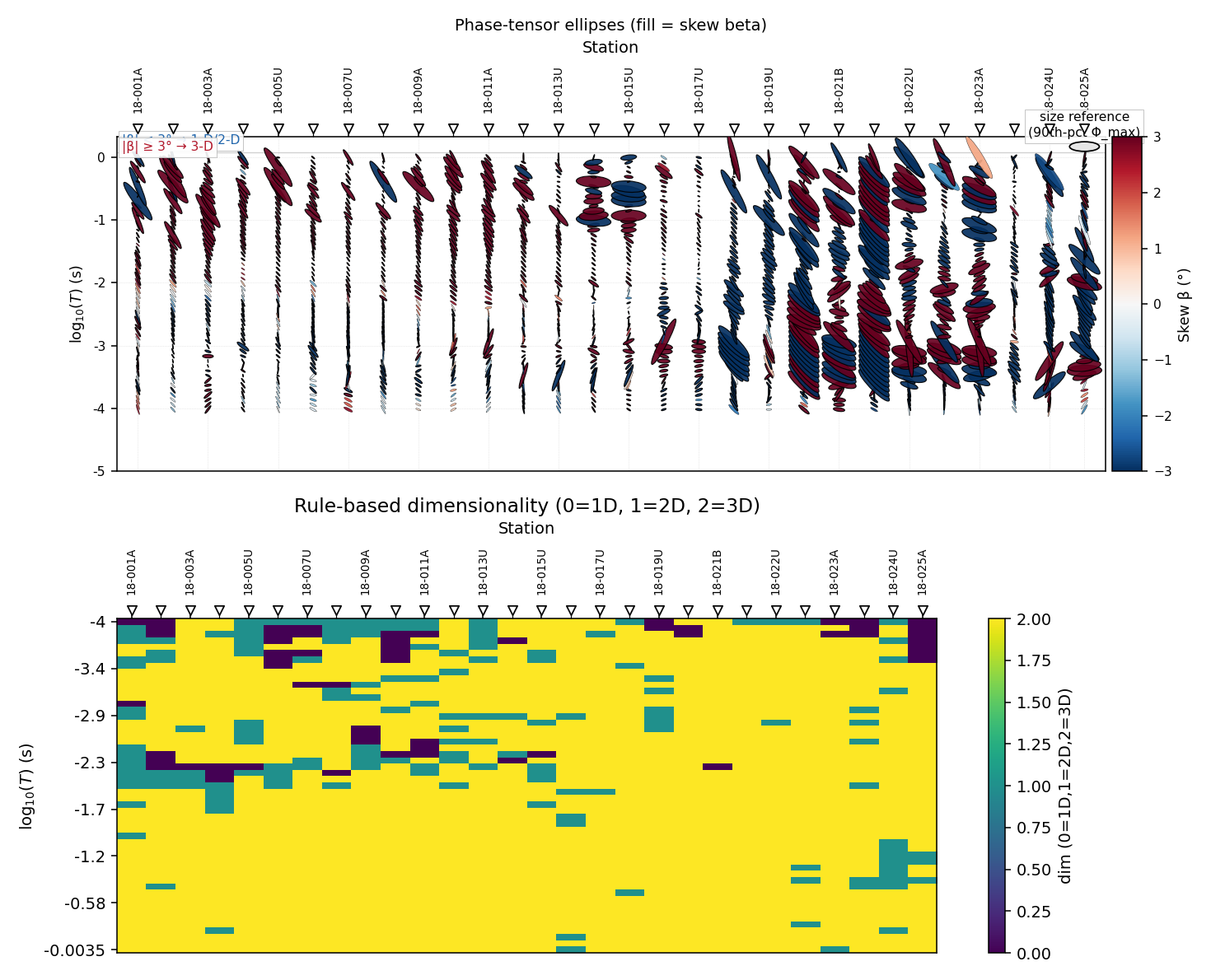
Top: ellipse shape encodes \(\phi_{\max}/\phi_{\min}\) (ellipticity) and orientation encodes \(\theta\); fill colour is skew \(\beta\). Bottom: the same data reduced to the three-way dimensionality label. The yellow (3-D) majority is concentrated station-wide, with pockets of teal (2-D) and a handful of purple (1-D) cells mostly at the shortest periods – exactly the pattern a near-surface, laterally heterogeneous overburden would produce on top of more consistent deeper structure.#
7.3. Groom-Bailey Galvanic Distortion#
Impedance Tensor already writes the static-shift distortion model as \(\mathbf{Z}_{obs}=\mathbf{C}\mathbf{Z}_{true}\) ((24)) for a diagonal gain-only \(\mathbf{C}\). Groom & Bailey (1989) [GroomBailey1989] generalize this to a full real 2x2 distortion matrix \(\mathbf{D}\) acting on a regional tensor \(\mathbf{Z}_{2D}\) that is assumed anti-diagonal after rotation to strike:
Because \(\mathbf{D}\) is real and frequency-independent while
\(\mathbf{Z}_{2D}\) carries all the frequency dependence, fitting
(4) across a band of frequencies over-determines
\(\mathbf{D}\) from a single station – that is the leverage that makes
the decomposition possible at all.
pycsamt.emtools.gb._fit_gb_distortion() solves it iteratively: given a
trial \(\mathbf{D}\), solve for the anti-diagonal
\(\mathbf{Z}_{2D}\) that best explains the observed \(\mathbf{Z}\),
then refit \(\mathbf{D}\) given that \(\mathbf{Z}_{2D}\), alternating
until the residual stabilizes.
The fitted \(\mathbf{D}\) is decomposed into four named parameters. Gain is its scale:
twist is the antisymmetric (rotational) part of the gain-normalized \(\mathbf{D}_n = \mathbf{D}/\mathrm{gain}\):
and shear and anisotropy come from rotating \(\mathbf{D}_n\) back by \(-\mathrm{twist}\) into \(\mathbf{M}=\mathbf{R}(-\mathrm{twist}) \mathbf{D}_n\) and reading its own symmetric/antisymmetric split:
There is a real, easy-to-miss consequence of (5) combined
with how _fit_gb_distortion() normalizes
\(\mathbf{D}\) at every iteration (to unit determinant, so the fit
doesn’t drift to an arbitrary scale): gain in
pycsamt.emtools.gb.groom_bailey_table() is not a free parameter at all,
it is pinned to \(1.0\) by construction, for every station, every time:
>>> from pycsamt.emtools.gb import groom_bailey_table
>>> gb = groom_bailey_table(sites)
>>> len(gb), (gb["status"] == "ok").sum()
(28, 28)
>>> round(float(gb["gain"].min()), 6), round(float(gb["gain"].max()), 6)
(1.0, 1.0)
This is not a bug – it is the classical Groom-Bailey scale ambiguity: an
overall multiplicative gain is indistinguishable from static shift
in this decomposition, so the fit deliberately normalizes it away and
reports only the shape parameters (twist, shear, anisotropy) that static
shift alone cannot produce. Any real amplitude scaling still present in the
data has to be handled separately, by the static-shift tools in
Static Shift, not read off this table’s gain column.
The other three parameters do vary station to station and carry real information:
>>> gb = gb.sort_values("station")
>>> round(float(gb["twist_deg"].abs().median()), 2)
11.72
>>> round(float(gb["shear"].abs().median()), 3)
0.236
>>> row0 = gb[gb["station"] == sites[0].station].iloc[0]
>>> [round(float(row0[k]), 4) for k in
...  ("twist_deg", "shear", "anisotropy", "rms_fit")]
[9.6171, -0.5186, 0.0756, 0.1607]
>>> round(float(gb["diagonal_ratio_before"].median()), 3), round(float(gb["diagonal_ratio_after"].median()), 3)
(0.423, 0.367)
Station 18-001A has a modest \(9.6^\circ\) twist and a shear of
\(-0.52\); across the whole line, median \(|{\rm twist}|\) is
\(11.7^\circ\) and median \(|{\rm shear}|\) is \(0.24\), both
comfortably nonzero – this line is not distortion-free. The median
diagonal/off-diagonal amplitude ratio drops from \(0.423\) before
correction to \(0.367\) after, a real but partial improvement, not a
clean collapse to zero.
“Partial” undersells how uneven that improvement is station by station.
Applying the fitted correction with
pycsamt.emtools.gb.groom_bailey_decomposition() and comparing
before/after diagonal ratios one station at a time shows the correction
working best exactly where distortion is mild, and making the diagonal
ratio worse at a cluster of high-twist, high-shear stations:
 1import matplotlib.pyplot as plt
 2import numpy as np
 3
 4x = np.arange(len(gb))
 5st = gb["station"].to_list()
 6fig, axes = plt.subplots(1, 3, figsize=(13.5, 4.2))
 7
 8axes[0].bar(x, gb["twist_deg"], color="#1f77b4")
 9axes[0].set_title("Twist (degrees)")
10
11axes[1].bar(x, gb["shear"], color="#d62728")
12axes[1].set_title("Shear (dimensionless)")
13
14axes[2].plot(x, gb["diagonal_ratio_before"], "o-", color="0.5", label="before GB")
15axes[2].plot(x, gb["diagonal_ratio_after"], "o-", color="#2ca02c", label="after GB")
16axes[2].set_title("Diagonal / off-diagonal ratio")
17axes[2].legend(fontsize=8)
18
19for ax in axes:
20    ax.set_xticks(x[::3])
21    ax.set_xticklabels([st[i] for i in x[::3]], rotation=45, ha="right", fontsize=7)
22    ax.grid(True, alpha=0.3)
23fig.tight_layout()
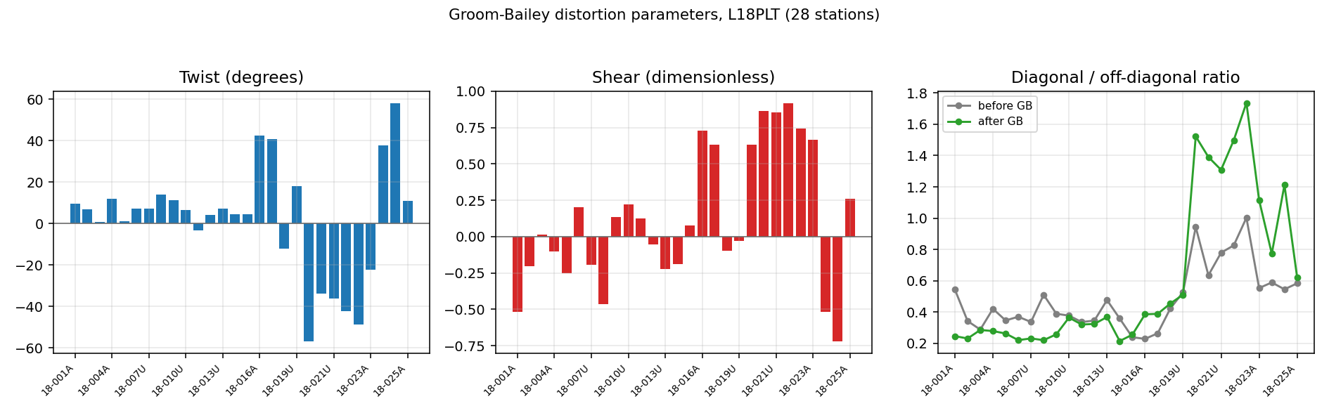
Twist and shear both grow sharply for the same run of stations
(18-020A through 18-024U, \(|\mathrm{twist}|\) up to
\(58^\circ\), \(|\mathrm{shear}|\) up to \(0.92\)). At those
same stations the green “after” curve sits
above the grey “before” curve – correcting for a fitted distortion
matrix made the residual diagonal terms larger, not smaller. 13 of the 28
stations end up worse by this measure, and it is not simply the stations
with the worst fit residual (rms_fit): the correlation between
rms_fit and the before/after change is only 0.17.#
The honest reading is that (4)’s core assumption – a single frequency-independent real \(\mathbf{D}\) explains the data on top of a purely anti-diagonal regional tensor – holds unevenly across this line. Where it holds, the correction genuinely suppresses diagonal energy. Where the underlying structure is not well described by any real distortion matrix over an anti-diagonal regional response (large, unstable twist/shear are the warning sign, not the fit residual alone), forcing the correction can inject as much diagonal energy as it removes. This is a standard, documented limitation of classical galvanic-distortion decomposition, not a pyCSAMT-specific defect – but it means station-by- station before/after comparison, not just the survey median, should guide whether to trust and apply a Groom-Bailey correction.
>>> from pycsamt.emtools.gb import groom_bailey_decomposition
>>> res = groom_bailey_decomposition(sites, apply=True)
>>> res.n_station, res.applied
(28, True)
GroomBaileyResult returns the corrected sites
alongside the fitted parameter table, ready for the same downstream steps
(static-shift review, strike estimation, dimensionality reclassification,
inversion) used elsewhere in this documentation.
7.4. Connection To Strike And Later Workflows#
The SVD orientation angle \(\theta\) returned alongside alpha/
beta in build_phase_tensor_table() is one
of the inputs pycsamt.emtools.strike.estimate_strike_consensus()
combines with other strike estimators; this page does not repeat that
material, which belongs to strike estimation specifically rather than
dimensionality classification. What this page adds is upstream of strike: a
reason to trust (or distrust) a 2-D/strike-based workflow in the first
place, and a distortion correction that can be applied before strike
rotation and inversion.
Dimensionality and Groom-Bailey diagnostics feed directly into:
Inversion Concepts, because 1-D/2-D/3-D dimensionality is a modelling choice made partly from the counts and figure above;
Static Shift, because Groom-Bailey’s gain-normalization means amplitude (static-shift) correction has to be handled separately, not read off the same table;
CSAMT, AMT, and MT Overview, which introduces phase tensor and skew as quick-look diagnostics without deriving them – this page is where that derivation lives.
7.5. Practical Guidance And Pitfalls#
Do not read
alphaas a skew orbetaas an orientation – confirm which is which for any pyCSAMT version by rotating a synthetic tensor, the same check that caught the swap described above.Treat
classify_dimensionality’s default thresholds (\(\text{skew\_th}=3^\circ\), \(\text{ellipt\_th}=0.2\)) as a screening rule, not a verdict – a majority-3-D result over a real survey is common and does not automatically disqualify a 2-D inversion.Do not average phase-tensor quantities across periods before checking whether the dimensionality label is stable with period; shallow and deep structure can classify differently at the same station.
Groom-Bailey’s
gaincolumn is always 1.0 by construction; look to static-shift tools, not this table, for amplitude correction.Always inspect the before/after diagonal ratio per station, not only the survey median, before trusting a Groom-Bailey correction – it can make individual stations worse even when the median improves.
Large, unstable twist or shear is itself diagnostic: it suggests the anti-diagonal regional-tensor assumption is breaking down, which is useful information even when the fit residual (
rms_fit) looks unremarkable.
7.6. References#
This page follows Caldwell, Bibby & Brown’s phase-tensor formulation [Caldwell2004] and Groom & Bailey’s galvanic-distortion decomposition [GroomBailey1989]. See also References.