11. Foundations of AI Inversion#

AI inversion does not remove the electromagnetic inverse problem. It changes how candidate earth models are proposed. A classical optimizer updates one model for one survey; a trained network learns a reusable mapping from data to model parameters. The same non-uniqueness, acquisition limits, error model, Maxwell physics, and geological assumptions remain. Understanding where each of those ingredients enters is essential before an AI-generated resistivity section can be interpreted scientifically.

This page develops that connection from the forward problem to validation. It complements Inversion Concepts, which introduces classical objectives, and the practical AI inversion workflows.

11.1. What the network actually learns#

Let \(\mathbf m\) contain log conductivity or log resistivity on a declared mesh, \(\mathcal F\) be the electromagnetic forward operator, and \(\mathbf d\) contain observed complex impedances or derived features. The measurement process is

(1)#\[\mathbf d_{obs}=\mathcal F(\mathbf m_{true})+\boldsymbol\epsilon,\]

where \(\boldsymbol\epsilon\) includes measurement noise, modelling error, and processing uncertainty. A neural inverter \(g_\theta\) produces

(2)#\[\widehat{\mathbf m}=g_\theta(\mathbf d_{obs}).\]

Equation (2) is an amortized inverse: the expensive learning stage is shared by later surveys. It is not the mathematical inverse of \(\mathcal F\). In most electromagnetic settings that inverse is neither unique nor stable.

To see why, consider a depth-sensitivity kernel whose scale follows pycsamt.forward.maxwell.skin_depth_m(). This is a transparent teaching proxy, not a replacement for a Maxwell solver:

>>> import numpy as np
>>> from pycsamt.forward.maxwell import skin_depth_m
>>> depth_m = np.linspace(25, 1975, 40)
>>> frequency_hz = np.geomspace(1, 1000, 14)
>>> delta = skin_depth_m(100.0, frequency_hz)
>>> kernel = np.exp(-depth_m[None, :] / delta[:, None])
>>> kernel /= kernel.sum(axis=1, keepdims=True)
>>> kernel.shape
(14, 40)

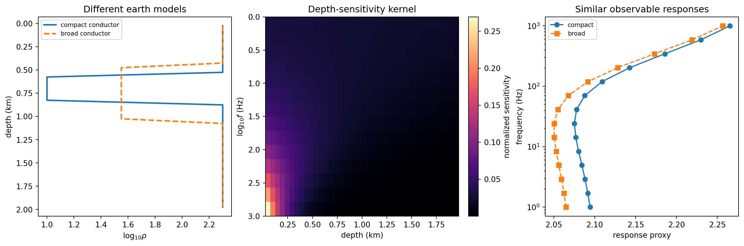
Different earth models, their depth sensitivity, and similar responses

The compact and broad conductors differ by 0.360 in model-space RMSE, yet their response-proxy RMSE is only 0.023. Low data misfit therefore does not prove correct geometry. The sensitivity panel also explains why shallow, high-frequency structure is usually better localized than deep structure: the rows of the forward map become broader with penetration depth.

11.2. Learning from known earth models#

In supervised AI inversion, synthetic pairs \(\{(\mathbf d_i,\mathbf m_i)\}_{i=1}^N\) are generated by drawing earth models and solving their responses,

(3)#\[\mathbf m_i\sim p_{train}(\mathbf m),\qquad \mathbf d_i=\mathcal F_h(\mathbf m_i)+\boldsymbol\epsilon_i.\]

The subscript \(h\) emphasizes that responses come from a discretized solver and mesh. The training distribution \(p_{train}\) is the operational meaning of the geological prior: it determines which layers, lenses, contacts, correlations, anisotropies, topographies, and resistivity contrasts the network can learn to recover.

The current geology API makes those assumptions explicit and reproducible:

>>> from pycsamt.ai.geology import (
...     ElectricalLayer, GaussianCorrelation, GeologyGrid,
...     generate_layered_geology,
... )
>>> grid = GeologyGrid.regular_2d(
...     nx=24, nz=16, dx_m=100, dz_m=75,
... )
>>> corr = GaussianCorrelation(700, 150)
>>> geology = generate_layered_geology(
...     grid,
...     [ElectricalLayer("cover", 30),
...      ElectricalLayer("host", 800)],
...     [450], seed=19,
...     interface_relief_std_m=60,
...     interface_correlation=corr,
... )
>>> geology.resistivity_ohm_m.shape, geology.seed
((16, 24), 19)

A fixed seed makes one realization repeatable, not representative. Scientific training varies the root seed and the geological hyperparameters, then checks whether validation and field features lie inside the resulting support.

11.2.1. Choosing the model coordinates#

The output coordinates determine what the network can express and how its errors are measured. Conductivity and resistivity are reciprocal,

(4)#\[\sigma(\mathbf x)=\rho(\mathbf x)^{-1},\]

so an arithmetic error in one is not an arithmetic error in the other. A positive resistivity is commonly represented by \(m=\log_{10}(\rho/\rho_0)\), where \(\rho_0=1\ \Omega\,\mathrm m\) is a reference used to make the logarithm dimensionless. The transformation

(5)#\[\rho(\mathbf x)=\rho_0,10^{m(\mathbf x)}\]

enforces positivity and prevents a few high-resistivity cells from dominating an unscaled linear-resistivity loss. It also gives an interpretable error: a model residual of \(0.3\) is approximately a factor-of-two resistivity error. Training, uncertainty, metrics, color limits, and exported arrays must all state whether they use \(\rho\), \(\sigma\), or \(\log_{10}\rho\); silently mixing them invalidates the comparison.

A cell model is also inseparable from its grid. For a 2-D section with \(n_z\) depth cells and \(n_x\) horizontal cells, \(\mathbf m\in\mathbb R^{n_z\times n_x}\). In 3-D it becomes \(\mathbf m\in\mathbb R^{n_z\times n_y\times n_x}\). An output merely indexed by station and depth has shape \(n_s\times n_z\); it may be a useful section or graph prediction, but it is not a voxel volume. This dimensional distinction should survive serialization rather than being inferred from an image after training.

11.2.2. The prior is an executable scientific hypothesis#

Uniform random pixels are rarely a credible geological prior. They contain abundant cell-scale discontinuities, whereas field geology is organized into interfaces, correlated domains, contacts, faults, intrusions, and bodies with finite extent. A network trained only on pixel noise can minimize synthetic loss while learning spatial statistics that have little relationship to an earth model.

Layered realizations start from ordered units. If interface \(k\) is described by a mean depth \(\bar z_k\) and a correlated displacement \(u_k(x)\), then

(6)#\[z_k(x)=\bar z_k+u_k(x),\qquad \operatorname{Cov}[u_k(x),u_k(x')] =s_k^2\exp\!\left[-\frac{(x-x')^2}{2\ell_{x,k}^2}\right].\]

Here \(s_k\) controls relief and \(\ell_{x,k}\) controls its horizontal continuity. Realizations must reject crossed interfaces or apply a documented repair; otherwise a nominally ordered stratigraphy can acquire negative layer thickness.

A finite target can be represented by a rotated ellipse in 2-D. With centre \((x_c,z_c)\), dip \(\varphi\), and semi-axes \(a_x,a_z\), define

(7)#\[\begin{split}\begin{aligned} x'&=(x-x_c)\cos\varphi+(z-z_c)\sin\varphi,\\ z'&=-(x-x_c)\sin\varphi+(z-z_c)\cos\varphi,\\ r_e^2&=\left(\frac{x'}{a_x}\right)^2+ \left(\frac{z'}{a_z}\right)^2. \end{aligned}\end{split}\]

Cells with \(r_e\leq1\) lie inside the lens. A transition shell blends in log-resistivity space, which preserves positivity and creates multiplicative rather than additive contrasts. Overlapping lenses require an explicit rule: first, last, most_conductive, most_resistive, or an error. The rule is part of the prior because it changes the frequency of composite targets.

>>> from pycsamt.ai.geology import EllipsoidalLens, insert_lenses
>>> ore = EllipsoidalLens(
...     "ore", center_x_m=1450, center_z_m=650,
...     radius_x_m=500, radius_z_m=140,
...     resistivity_ohm_m=8, dip_deg=18,
...     transition_fraction=0.2,
... )
>>> with_body = insert_lenses(
...     geology, [ore], conflict_policy="most_conductive",
... )
>>> with_body.lens_index.shape
(16, 24)
>>> int((with_body.lens_index >= 0).sum())
29

The body count, size distribution, contrast, dip, transition width, and chance of no target should all vary across the ensemble. If every training example contains a centered conductor, the network is rewarded for placing one there even when the observations do not require it. Negative examples are therefore as important as spectacular targets.

11.2.3. Topography changes cells, not just plotting coordinates#

Let \(h(x)\) be elevation and \(h_{ref}\) the elevation assigned to depth zero. The terrain depth is

(8)#\[z_s(x)=h_{ref}-h(x),\]

and a cell centre belongs to earth when \(z\geq z_s(x)\). This produces an active-earth mask \(A(z,x)\). Air cells must be excluded from earth-model losses and assigned the conductivity required by the forward solver. Merely warping the top edge of a rectangular inversion image changes neither Maxwell physics nor training support.

>>> from pycsamt.ai.geology import TopographicSurface
>>> elevation = [410, 425, 432, 421, 405, 398, 407, 419,
...              431, 440, 429, 417, 408, 402, 411, 423,
...              435, 442, 430, 418, 409, 401, 406, 414]
>>> terrain = TopographicSurface(
...     grid, elevation, reference_elevation_m=442,
...     source="survey stations",
... )
>>> terrain.relief_m
44.0
>>> terrain.earth_mask().shape
(16, 24)

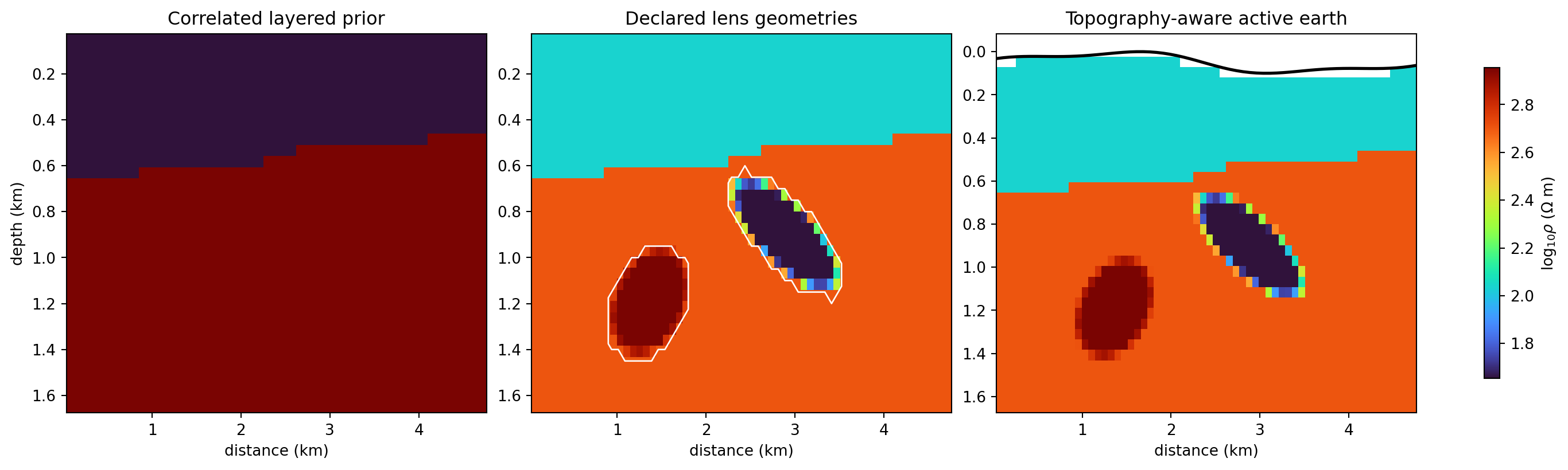
Layered geological prior, embedded lenses, and topographic active cells

The left panel contains a continuous interface rather than independent pixels. The centre panel adds bodies whose white outlines expose the declared geometry; the conductive dipping lens and resistive body are not post-processing effects. The right panel applies the terrain-derived mask. Blank cells are air and are not permissible places for geological recovery scores. Together the panels show that “the prior” is a composition of auditable choices, not one smoothness constant.

11.2.4. Sampling the prior without leaking the answer#

Every realization needs an identity derived before splitting. Variants of the same base geology, noise draw, or forward response must remain in one split. Otherwise the test set measures recognition of a near duplicate rather than generalization. A useful hierarchy is

(9)#\[s_{i,q}=H(s_0,\,i,\,q),\]

where \(s_0\) is the experiment seed, \(i\) the realization identifier, \(q\) a named random process such as interfaces, lenses, or noise, and \(H\) a stable seed derivation. Naming the process prevents adding a new random draw from silently changing all subsequent draws.

Prior coverage should be inspected in parameter and response space. Histograms of resistivity, target depth, body aspect ratio, relief, and correlation length find obvious omissions. Response features then reveal less obvious collapse: many distinct parameter draws can occupy the same narrow electromagnetic support, or apparently moderate parameter ranges can generate extreme phase behavior. Both views are needed before expensive training begins.

11.3. Maxwell physics belongs inside the evidence chain#

For frequency-domain electromagnetics, neglecting displacement current in a conductive earth gives a curl–curl equation such as

(10)#\[\nabla\times\mu^{-1}\nabla\times\mathbf E +i\omega\sigma(\mathbf x)\mathbf E =\mathbf s,\]

with a documented time convention, boundary treatment, source, receiver interpolation, and active-cell mask. A training label is physically grounded only when its response is computed by a solver whose capability contract covers the requested dimension, components, mesh, and topography.

The updated Maxwell boundary constructs that numerical problem separately from the neural network:

>>> import numpy as np
>>> from pycsamt.forward.maxwell import MeshDesign, build_solver_mesh
>>> solver_model = build_solver_mesh(
...     grid,
...     resistivity_ohm_m=geology.resistivity_ohm_m,
...     frequencies_hz=[100, 10, 1],
...     design=MeshDesign(
...         horizontal_padding_cells=3,
...         bottom_padding_cells=4,
...         air_layers=3,
...     ),
... )
>>> solver_model.mesh.dimension, solver_model.conductivity_s_m.shape
(2, (23, 30))
>>> solver_model.quality.cell_count
690

Padding, air, topography, and quality warnings are part of the forward model; draping a finished image onto terrain is not. Likewise, a station-by-layer graph prediction is not a voxelwise 3-D Maxwell inversion. The solver capability report must pass before a physics residual is treated as evidence.

11.3.1. Discretization defines the physics that is learned#

The continuous equation (10) is replaced by a discrete system

(11)#\[\mathbf A_h(\mathbf m,\omega)\mathbf e =\mathbf q,\]

where \(\mathbf A_h\) depends on cell geometry, material averaging, boundary conditions, and frequency. Receiver interpolation then produces \(\mathbf d=\mathbf P\mathbf e\). Consequently, a neural network trained with one discretization learns both earth physics and the numerical signature of that discretization. Mesh-convergence tests and a second solver, when available, help separate those effects.

Cell dimensions should resolve the smallest relevant skin depth and geological feature without making the domain too small at low frequency. A common planning scale in a uniform half-space is

(12)#\[\delta(f,\rho)\approx503 \sqrt{\frac{\rho\,[\Omega\,\mathrm m]}{f\,[\mathrm{Hz}]}}\ \mathrm m.\]

This is a scale estimate, not a mesh guarantee. Strong contrasts, topography, anisotropy, receiver placement, and the numerical formulation can demand finer cells. Padding should grow away from the survey so artificial boundaries do not control the response, while cell growth must remain gradual enough for the chosen backend.

The dataset contract binds every model to its frequencies, receivers, components, mesh provenance, split, and solver diagnostics. The configuration can be validated without launching the expensive solve:

>>> import numpy as np
>>> from pycsamt.ai.training.dataset2d import Maxwell2DDatasetConfig
>>> training_grid = GeologyGrid.regular_2d(
...     nx=20, nz=14, dx_m=150, dz_m=100,
... )
>>> dataset_config = Maxwell2DDatasetConfig(
...     dataset_id="regional-2d-v1",
...     grid=training_grid,
...     correlation_length_x_m=(300, 1200),
...     correlation_length_z_m=(100, 400),
...     frequencies_hz=np.geomspace(1, 1000, 16),
...     station_x_m=np.linspace(225, 2775, 12),
...     n_realizations=240,
...     seed=2028,
...     validation_fraction=0.15,
...     test_fraction=0.15,
... )
>>> dataset_config.components
('zxy', 'zyx')
>>> len(dataset_config.frequencies_hz), dataset_config.n_realizations
(16, 240)

The example uses 240 realizations and 16 frequencies because a demonstration with two realizations cannot establish structural recovery. These values are starting points, not universal minima. Increase realizations when the prior contains more facies, body families, fault styles, or acquisition patterns; increase retained frequencies only when they add reliable, non-redundant sensitivity. A reproducible learning curve—validation error versus number of realizations—is more informative than quoting one dataset size.

Survey geometry cannot be treated as an incidental tensor length. If a network expects fixed station positions, applying it to a different spacing changes the meaning of each input index. Options include resampling onto a declared common coordinate, encoding coordinates as inputs, using masks with a geometry-aware architecture, or training separate acquisition families. Each option adds a different interpolation or inductive assumption and must be tested on held-out geometries.

Complex impedance should remain complex until a documented feature transform. For the convention \(Z=E/H\), apparent resistivity and phase are

(13)#\[\rho_a=\frac{|Z|^2}{\mu_0\omega},\qquad \phi=\operatorname{atan2}(\Im Z,\Re Z).\]

Predicting or normalizing phase requires circular care near its branch cut. Training on real and imaginary impedance preserves linear residual structure, whereas apparent resistivity and phase can be easier to visualize. Neither is intrinsically correct for every architecture; what matters is that the forward response, observed tensor, error tensor, and inverse transform share an exact contract.

11.3.2. Noise should resemble the survey, not decorate it#

Independent Gaussian noise is useful for controlled tests but is rarely a complete field error model. A synthetic observation may be written

(14)#\[\widetilde Z_{sfc}=Z_{sfc} +\eta^{rel}_{sfc}|Z_{sfc}| +\eta^{floor}_{sfc} +b_{sc}Z_{sfc},\]

where the first term represents relative random error, the second an absolute noise floor, and \(b_{sc}\) a station/component systematic effect. Missing frequencies, dead components, coherent distortion, and station-dependent error floors should be simulated when they occur in the application. The validity mask must distinguish an absent datum from a numerical zero.

Noise augmentation belongs after the train/validation/test split or must use a split-specific seed. Otherwise two noisy versions of one noiseless response can leak across the boundary. Validation should include both familiar noise and deliberately shifted noise so robustness is measured rather than assumed.

11.4. Why the objective needs several terms#

A useful training or refinement objective separates model recovery, response fit, regularization, and geological constraints:

(15)#\[\mathcal J(\theta)= \lambda_m\,\mathcal L_m(g_\theta(\mathbf d),\mathbf m) +\lambda_d\left\|\mathbf W_d [\mathcal F_h(g_\theta(\mathbf d))-\mathbf d]\right\|_2^2 +\lambda_s\mathcal R(g_\theta(\mathbf d)) +\lambda_g\Phi_g(g_\theta(\mathbf d)).\]

\(\mathcal L_m\) teaches known-model recovery. The response term asks whether the predicted earth explains the data under their errors. \(\mathcal R\) controls unstable spatial variation, while \(\Phi_g\) expresses declared geological information. Their weights are not aesthetic controls: increasing smoothness can lower variance while erasing a narrow conductor, and a strong prior can manufacture a geologically familiar feature unsupported by observations.

The loss must be evaluated in consistent spaces. For complex impedance \(Z\), a scale-aware residual may be written

(16)#\[r_{sfc}=\frac{Z^{pred}_{sfc}-Z^{obs}_{sfc}} {\max(\sigma_{sfc},\sigma_{floor})},\]

where \(s,f,c\) index station, frequency, and component. A single global RMS can hide a failed component, depth interval, or target boundary, so retain the residual tensor and its aggregation policy.

11.4.1. Model-space losses answer different questions#

For valid cells \(p\in\mathcal V\), let \(e_p=\widehat m_p-m_p\). The familiar pointwise losses are

(17)#\[\mathcal L_1=\frac{1}{|\mathcal V|}\sum_{p\in\mathcal V}|e_p|, \qquad \mathcal L_2=\frac{1}{|\mathcal V|}\sum_{p\in\mathcal V}e_p^2,\]

and the Huber penalty is

(18)#\[\begin{split}h_\delta(e)= \begin{cases} \tfrac12e^2,&|e|\leq\delta,\\ \delta(|e|-\tfrac12\delta),&|e|>\delta. \end{cases}\end{split}\]

L2 strongly emphasizes large errors and is appropriate when residuals are approximately Gaussian and severe misses should dominate. L1 has constant influence away from zero and better resists rare corrupted labels. Huber is quadratic near zero but linear for large residuals. Its threshold must be set in the model coordinates: delta=0.5 in log10 resistivity has a very different physical meaning from delta=0.5 ohm metre.

>>> import numpy as np
>>> from pycsamt.ai.losses import (
...     model_huber_loss, model_l1_loss, model_l2_loss,
... )
>>> residual_case = np.array([0.0, 0.1, -0.1, 3.0])
>>> target = np.zeros_like(residual_case)
>>> round(model_l1_loss(residual_case, target).value, 3)
0.8
>>> round(model_l2_loss(residual_case, target).value, 3)
2.255
>>> round(model_huber_loss(
...     residual_case, target, delta=0.5,
... ).value, 3)
0.347

The three numbers use the same four errors. The isolated residual 3.0 controls L2, while Huber retains sensitivity without allowing that cell to overwhelm all smaller errors. Robustness is not permission to ignore why an outlier exists; it prevents one bad label from determining every update while the label is audited.

11.4.2. Depth weights change the estimand#

Electromagnetic sensitivity generally decays and broadens with depth. Uniform cell averaging can also let a large deep region dominate the count even when its cells are weakly constrained. With non-negative weights \(w_p\), the weighted model loss is

(19)#\[\mathcal L_{m,w}= \frac{\sum_{p\in\mathcal V}w_p\,\ell(e_p)} {\sum_{p\in\mathcal V}w_p}.\]

Weights may balance depth intervals, target/background cells, or facies. They do not create sensitivity. Heavy deep weighting can force a network to match synthetic deep priors even where the data contain little information, producing precise-looking but prior-driven structure.

>>> from pycsamt.ai.losses import depth_weights, model_l2_loss
>>> weights_z = depth_weights(4)
>>> np.round(weights_z, 3).tolist()
[0.48, 0.24, 0.16, 0.12]
>>> pred = np.array([[2.1, 2.2], [2.0, 2.2],
...                  [2.7, 2.9], [3.0, 3.2]])
>>> true = np.full_like(pred, 2.0)
>>> weighted = model_l2_loss(
...     pred, true, weights=weights_z[:, None],
... )
>>> round(weighted.value, 3), weighted.n_valid
(0.226, 8)

The returned n_valid and weight sum are provenance, not decoration. They make a loss comparable across batches with different masks and prevent an apparently small value caused by evaluating only a few cells.

11.4.3. Smoothness and total variation encode structure#

On a grid, directional first differences are

(20)#\[(D_xm)_{j,i}=m_{j,i+1}-m_{j,i},\qquad (D_zm)_{j,i}=m_{j+1,i}-m_{j,i}.\]

Quadratic smoothness penalizes \(\|D_xm\|_2^2+\|D_zm\|_2^2\) and therefore favors gradual transitions. Anisotropic total variation uses

(21)#\[\operatorname{TV}(m)= \sum_{j,i}|(D_xm)_{j,i}|+ \sum_{j,i}|(D_zm)_{j,i}|,\]

which permits a smaller number of sharp contacts. Neither is neutral. A smoothness penalty can widen a thin conductor until its contrast weakens; TV can staircase a genuinely graded alteration halo.

>>> from pycsamt.ai.losses import (
...     gradient_smoothness_loss, total_variation_loss,
... )
>>> section = np.array([[2.5, 2.5, 1.0, 1.0],
...                     [2.5, 2.4, 1.1, 1.0]])
>>> gx = gradient_smoothness_loss(
...     section, axis=1, kind="l2",
... )
>>> tv = total_variation_loss(section, kind="l1")
>>> round(gx.value, 3), round(tv.value, 3)
(0.71, 0.5)

Cell spacing matters when the grid is nonuniform. A difference penalty without division by physical spacing penalizes change per cell, not gradient per metre. Likewise, area or volume weights may be necessary if cell sizes vary. The implemented array losses expose the elemental arithmetic; the experiment must declare any geometry-aware weights used around it.

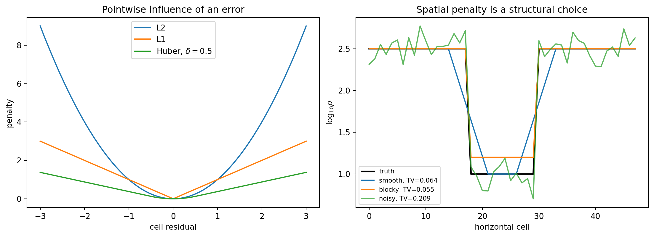
L1, L2, and Huber influence curves and total variation of model profiles

The left panel shows why one outlier bends an L2 objective much more strongly than L1 or Huber. The right panel reveals a different issue: the smooth and blocky profiles can both have modest TV, while cell-scale noise is expensive. The penalty removes oscillation but cannot decide whether the true contact is sharp or gradual; that decision needs prior knowledge and held-out recovery.

11.4.4. Boundary losses make inactive regions explicit#

If \(B_p\) selects air or fixed padding cells and \(m_B\) is their required value, a boundary penalty is

(22)#\[\mathcal L_B= \frac{\sum_pB_p\,\ell(\widehat m_p-m_{B,p})}{\sum_pB_p}.\]

The target cannot be implicit because air conductivity, log-resistivity encoding, and solver conventions differ. Earth cells should not accidentally contribute to this term.

>>> from pycsamt.ai.losses import boundary_condition_loss
>>> predicted = np.array([[7.5, 7.8, 8.0],
...                       [2.0, 2.1, 2.2]])
>>> air = np.array([[True, True, True],
...                 [False, False, False]])
>>> result = boundary_condition_loss(
...     predicted, boundary_mask=air,
...     target=8.0, kind="l1",
... )
>>> round(result.value, 3), result.n_valid
(0.233, 3)

11.4.5. Response losses reconnect the proposal to observations#

Model loss alone teaches resemblance to one sampled truth, even though another model may explain the response equally well. Response consistency evaluates the proposal under \(\mathcal F_h\). With complex standard errors \(s_{sfc}>0\), the implemented L2 form averages squared complex normalized residual magnitude,

(23)#\[\mathcal L_d=\frac1{|\mathcal O|} \sum_{(s,f,c)\in\mathcal O} \left| \frac{Z^{pred}_{sfc}-Z^{obs}_{sfc}}{s_{sfc}} \right|^2.\]

>>> from pycsamt.ai.losses import response_residual_loss
>>> observed = np.array([1+2j, 2+1j])
>>> predicted = np.array([1.1+2.2j, 1.8+1.1j])
>>> errors = np.array([0.2, 0.25])
>>> response_fit = response_residual_loss(
...     predicted, observed, errors=errors,
... )
>>> round(response_fit.value, 3), response_fit.normalized
(1.025, True)

Exact station, frequency, and component alignment is required. Reordering or interpolating inside the loss can produce an attractive scalar from mismatched observations. Use the contract-aware loss when working with ForwardResult and SurveyData so incompatible axes fail loudly.

11.4.6. Choosing the weights is an experiment#

Raw magnitudes of the terms in (15) depend on reduction, units, mask size, and batch composition. Setting every \(\lambda\) to one does not make their scientific influence equal. A disciplined procedure is:

record unweighted term values and gradient norms on the same initial batch;
normalize only where the statistical meaning supports it;
sweep a small, predeclared range of weights;
compare the Pareto trade-off between response fit and structural recovery;
select on validation realizations, never the field image;
freeze the weights before final test evaluation.

If increasing \(\lambda_d\) improves response fit but worsens known-target geometry, the forward term may be exploiting non-uniqueness or solver artifacts. If increasing \(\lambda_g\) improves visual plausibility without improving response or recovery, the prior is dominating. Those trade-offs are results to report, not nuisances to conceal in one total-loss curve.

11.5. Supervised, hybrid, and physics-informed routes#

The same scientific ingredients can be arranged in different optimization routes. A supervised network minimizes model loss over a dataset and is fast at inference. A hybrid method uses that network as a proposal, then refines the model against the observed response. A physics-informed neural network places differential-equation residuals directly in training. These routes are related but not interchangeable.

For supervised learning, empirical risk minimization is

(24)#\[\widehat\theta=arg\min_\theta \frac1{N_{tr}}\sum_{i\in\mathcal I_{tr}} \mathcal L\!\left(g_\theta(\mathbf d_i),\mathbf m_i\right).\]

The validation split selects architecture, early stopping, and hyperparameters; the test split is used once for an unbiased final estimate. Batch sampling should not allow common easy background models to overwhelm rare target families. Stratification or explicit sample weights can balance that exposure, but the natural prevalence needed for deployment should still be represented in a separate evaluation.

11.5.2. Physics-informed neural networks#

A PINN represents fields, material parameters, or both with neural functions and evaluates Maxwell residuals at collocation points. If \(\mathbf E_\theta(\mathbf x,\omega)\) is a learned electric field and \(\sigma_\psi(\mathbf x)\) a learned conductivity, an interior residual is

(26)#\[\mathbf r_\Omega= \nabla\times\mu^{-1}\nabla\times\mathbf E_\theta +i\omega\sigma_\psi\mathbf E_\theta-\mathbf s.\]

Training may combine

(27)#\[\mathcal L_{PINN}= \lambda_\Omega\frac1{N_\Omega}\sum_{q=1}^{N_\Omega} \|\mathbf r_\Omega(\mathbf x_q)\|_2^2 +\lambda_B\mathcal L_B +\lambda_d\mathcal L_d.\]

Automatic differentiation makes spatial derivatives available, but it does not guarantee a physically correct solution. The field representation must handle complex values, sources and singular behavior; collocation points must resolve interfaces; boundary conditions must be complete; and residual units must be scaled. A tiny collocation residual between sparse points can coexist with a poor receiver response. Benchmark a PINN against an accepted numerical solver on canonical half-spaces and layered models before using its residual as an inversion constraint.

11.5.3. Graph networks and irregular surveys#

A graph network is attractive when stations are irregular. Define nodes at station coordinates and connect nearby pairs, for example with

(28)#\[A_{ij}=\mathbb 1(\|\mathbf x_i-\mathbf x_j\|\leq r) \exp\!\left[-\frac{\|\mathbf x_i-\mathbf x_j\|^2}{2\ell_g^2}\right].\]

A message-passing layer can then update node features by

(29)#\[\mathbf h_i^{(l+1)}=\phi_l\!\left( \mathbf h_i^{(l)}, \sum_{j\in\mathcal N(i)}A_{ij}\, \psi_l(\mathbf h_i^{(l)},\mathbf h_j^{(l)},\mathbf e_{ij}) \right).\]

Coordinate differences, topography, component masks, and frequency features can enter \(\mathbf e_{ij}\) or node attributes. The radius and normalization must be stable when station density changes. Most importantly, output geometry defines the claim: node-by-depth predictions remain station columns even when the graph uses 3-D coordinates. Calling such an output “3-D inversion” would overstate what was recovered.

11.5.4. Architectures should respect missingness#

Zero-filled impedance is ambiguous because zero could be a valid transformed value. Supply a validity mask and, where appropriate, uncertainty or error features. During training, randomly mask realistic frequency bands and components so the model learns graceful degradation. Validation should plot recovery against the fraction and pattern of missing data. Random individual dropout alone does not emulate losing an entire high-frequency band or one polarization.

Output activations also carry assumptions. A linear log-resistivity head has unbounded support; clipping after inference can pile probability on artificial limits. A bounded transform guarantees a declared range but cannot extrapolate beyond it. Report how often predictions approach bounds, because saturation is an OOD diagnostic rather than merely a plotting inconvenience.

11.6. The domain gap is a scientific variable#

The domain gap is the difference between the synthetic joint distribution used for learning and the field distribution to which the model is applied. It includes more than noise: dimensionality, station spacing, frequency coverage, component availability, topography, distortion, geological scale, and solver discrepancy all contribute.

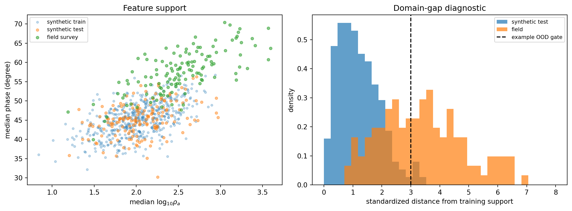
Synthetic and field feature support with an out-of-distribution score

Here the synthetic test set remains near training support with median distance 1.04, whereas the field median is 3.35 and lies beyond the illustrative OOD gate. A confident prediction in that region is extrapolation. The correct response is to revise the simulator, preprocessing, or applicability claim—not to interpret the model more confidently.

No single OOD score proves compatibility. Marginal range checks find a field frequency or phase outside every training example, while multivariate distances find unusual combinations. Learned embeddings can expose differences hidden in summary features, but their geometry depends on the trained network. Use several diagnostics and calibrate thresholds on held-out synthetic shifts whose severity is known.

Domain randomization deliberately widens nuisance variables—noise levels, station offsets, topography, distortion, and solver settings—so the inverse map cannot rely on one synthetic signature. Excessive randomization can make the task unnecessarily ambiguous and reduce accuracy in the intended domain. Targeted randomization begins from field quality-control summaries and broadens only uncertainties that are defensible.

Fine-tuning on field data requires labels or a trustworthy self-supervised objective. Reusing the observed response as both adaptation signal and final evidence creates optimistic assessment. Keep surveys, lines, or spatial blocks held out at the highest independent level and preserve a synthetic known-truth benchmark so adaptation cannot silently destroy recovery.

11.7. Uncertainty must be calibrated against error#

Predictive uncertainty combines irreducible data ambiguity and uncertainty in the learned mapping. For ensemble members or posterior samples \(\widehat{\mathbf m}^{(k)}\), a simple decomposition begins with

(30)#\[\bar{\mathbf m}=\frac1K\sum_{k=1}^K\widehat{\mathbf m}^{(k)},\qquad \mathbf s_m^2=\frac1{K-1}\sum_{k=1}^K (\widehat{\mathbf m}^{(k)}-\bar{\mathbf m})^2.\]

The map \(\mathbf s_m\) is useful only after calibration. On synthetic truth, an interval with nominal coverage \(1-\alpha\) should satisfy

(31)#\[\operatorname{coverage}_{1-\alpha}= \frac1P\sum_{p=1}^{P} \mathbb 1\!\left[m_p\in [q_{\alpha/2,p},q_{1-\alpha/2,p}]\right].\]

Overly broad intervals can achieve high coverage while being uninformative; narrow intervals can look decisive while missing truth. Report coverage with interval width and depth- or target-resolved error.

11.7.1. Aleatoric and epistemic uncertainty#

Aleatoric uncertainty represents ambiguity conditional on the inputs, including measurement noise and unresolved equivalence. Epistemic uncertainty represents limited knowledge of the mapping caused by finite data, architecture, or optimization. If member \(k\) predicts mean \(\boldsymbol\mu_k\) and variance \(\mathbf v_k\), the law of total variance gives

(32)#\[\operatorname{Var}(\mathbf m\mid\mathbf d) \approx \underbrace{\frac1K\sum_{k=1}^K\mathbf v_k}_{\text{aleatoric}} +\underbrace{\frac1K\sum_{k=1}^K (\boldsymbol\mu_k-\bar{\boldsymbol\mu})^2}_{\text{epistemic}}.\]

Independent seeds should vary initialization and data order; a stronger ensemble also varies plausible prior and noise configurations. Members trained on exact copies of one narrow dataset underestimate epistemic uncertainty under domain shift.

A heteroscedastic Gaussian output can learn a cellwise log variance \(a_p=\log v_p\) with negative log likelihood

(33)#\[\mathcal L_{NLL}=\frac1{2|\mathcal V|} \sum_{p\in\mathcal V} \left[e_p^2\exp(-a_p)+a_p+\log(2\pi)\right].\]

The first term rewards accurate means relative to predicted variance, while the second prevents variance from growing without cost. Gaussianity may be a poor description of a multimodal inverse problem: one broad interval between two distinct geological alternatives can describe neither alternative well.

>>> from pycsamt.ai.losses import gaussian_nll_loss, calibration_loss
>>> mean = np.array([2.0, 1.4, 2.5])
>>> truth = np.array([2.1, 1.0, 2.4])
>>> log_variance = np.log(np.array([0.04, 0.16, 0.09]))
>>> nll = gaussian_nll_loss(mean, truth, log_variance)
>>> round(nll.value, 3)
-0.097
>>> empirical = np.array([0.48, 0.77, 0.91])
>>> nominal = np.array([0.50, 0.80, 0.95])
>>> round(calibration_loss(empirical, nominal).value, 4)
0.001

A negative Gaussian NLL is possible for densities narrower than unit scale; it is not an error. Its absolute value depends on units and parameterization, so compare like with like. The calibration value summarizes deviations at chosen levels but does not show their direction. Plot empirical against nominal coverage and report interval widths.

Uncertainty should respond to controlled degradation. Remove high frequencies, increase noise, shift station geometry, and move geological parameters toward the edge of training support. Error and uncertainty should rise together. If error increases while reported uncertainty remains flat, the uncertainty model has failed precisely where it is most needed.

11.8. Validation decides whether interpretation is allowed#

Known-truth recovery provides evidence that field data cannot. The validation API reports global and depth-resolved errors:

>>> import numpy as np
>>> from pycsamt.ai.validation import recovery_report
>>> truth = np.array([[2.0, 1.0], [2.5, 2.5]])
>>> prediction = np.array([[2.1, 1.3], [2.4, 2.6]])
>>> report = recovery_report(prediction, truth, compute_ssim=False)
>>> round(report.rmse, 3), round(report.mae, 3)
(0.187, 0.15)
>>> np.round(report.depth_rmse, 3).tolist()
[0.224, 0.1]

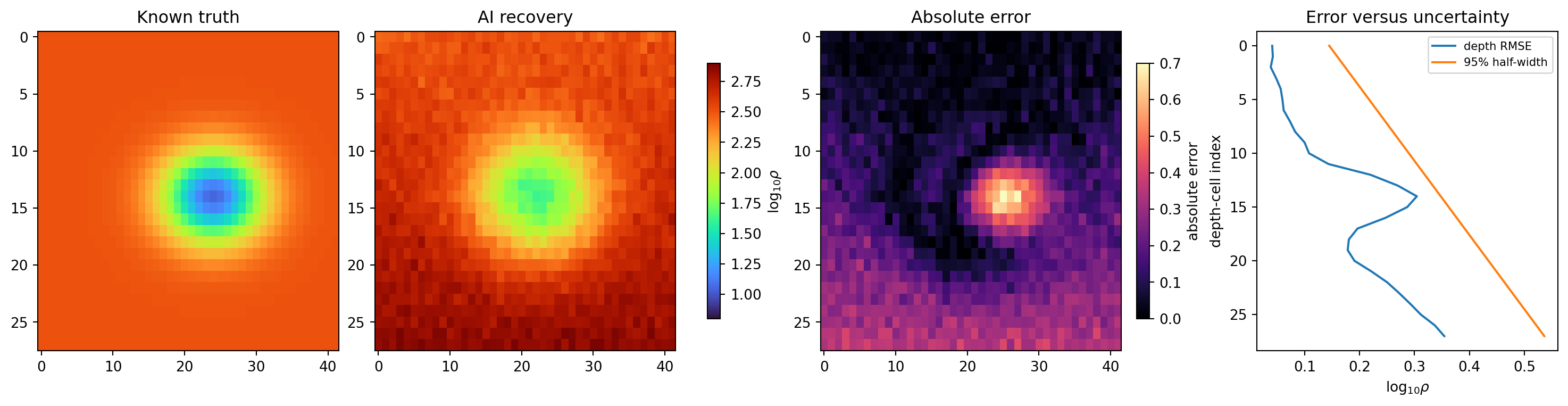
Known truth, AI recovery, spatial error, and depth uncertainty

The example recovery has RMSE 0.205 but only \(R^2=0.373\); its smoothed, shifted body loses substantial structural information. Nominal 95% coverage is 0.978, which is conservative rather than automatically good. The depth panel shows why scalar metrics are insufficient: error and interval width both increase downward.

A defensible promotion decision combines, at minimum, held-out recovery, response residuals, OOD screening, uncertainty calibration, seed stability, and comparison with a simpler baseline. Thresholds must be chosen for the declared use before inspecting the field image. Passing a software run or a single RMS threshold is not equivalent to scientific validation.

11.8.1. Structural recovery needs structural metrics#

RMSE and MAE measure cellwise amplitude but do not directly measure location, extent, or connectivity. For a target mask \(T\) and predicted mask \(\widehat T\), intersection over union is

(34)#\[\operatorname{IoU}(T,\widehat T)= \frac{|T\cap\widehat T|}{|T\cup\widehat T|}.\]

Centroid error, top/base depth error, recovered thickness, contrast ratio, and connected-component count answer complementary geological questions. The threshold used to create \(\widehat T\) must be predeclared or swept on validation data, not chosen separately for every attractive result.

Background cells often vastly outnumber target cells. A model that predicts only background can therefore have a reassuring global RMSE. Report metrics for target, near-target halo, background, and depth bands. Where a body family is sometimes absent, include false-positive rate on those negative examples.

Response validation should retain the data axes. For each frequency and component, inspect normalized residual median, spread, and station pattern. Coherent residuals across adjacent stations indicate structure the model does not explain; alternating residuals may indicate station-specific processing or an overly rough prediction. A global value erases that diagnostic geometry.

11.8.2. Splits should test the intended claim#

A random realization split tests interpolation within one simulator family. Stronger tests hold out geological families, acquisition geometries, noise regimes, frequency bands, or entire spatial regions. The appropriate hierarchy depends on the deployment claim:

interpolation test: new seeds inside trained parameter ranges;
compositional test: familiar layers and bodies in unseen combinations;
geological shift test: held-out fault, lens, or correlation regimes;
acquisition shift test: unseen station spacing or missing bands;
solver shift test: responses from a different validated discretization;
field transfer test: an independent survey with external evidence.

Success on the first does not imply success on the last. Report them separately so a useful interpolation model is not rejected merely for limited scope, and also not promoted beyond that scope.

Seed stability tests optimization uncertainty. For metric \(M_k\) from seed \(k\), report its distribution and a robust spread such as

(35)#\[\operatorname{IQR}(M)=Q_{0.75}(M)-Q_{0.25}(M).\]

The best seed is not a performance estimate. Publish the selection rule and all evaluated seeds; if an ensemble is the deployed estimator, evaluate the ensemble itself rather than substituting its strongest member.

11.8.3. Learning curves separate data and model limitations#

Plot training and validation loss against optimization step, but also plot held-out recovery against number of realizations. If training loss improves while validation worsens, regularization, augmentation, or early stopping may help. If both plateau at poor recovery, the architecture, inputs, resolution, or non-uniqueness may be limiting. If performance improves steadily with more realizations, the honest next step is more representative simulation rather than a more elaborate network.

Validation-based early stopping chooses the checkpoint

(36)#\[t^*=\arg\min_{t\in\mathcal T} \left[\mathcal L_{val}(t)+\kappa\,C_{val}(t)\right],\]

where \(C_{val}\) may be a structural or calibration penalty and \(\kappa\) is fixed in advance. Selecting solely by total training loss can prefer a checkpoint with worse target recovery. The test set remains untouched until \(t^*\) and all weights are frozen.

11.8.4. Baselines expose whether AI adds evidence#

At minimum compare with a constant or layered predictor, a simple regression baseline, and an established deterministic inversion where available. The AI method should improve a declared outcome—speed at comparable quality, structural recovery, robustness, or uncertainty—not merely produce a different image. Forward-evaluate every candidate through the same solver and error model to keep the comparison fair.

11.9. Failure patterns and their interpretation#

Several visual patterns recur and have specific scientific implications:

A central conductor in most outputs often reflects centered targets in the prior or padding/alignment leakage. Check negative examples and translate the survey laterally.
Identical-looking sections for different lines can indicate collapsed training, overly aggressive normalization, constant features, or a prior that overwhelms the inputs. Compare raw feature statistics and a shuffled-input prediction.
A smooth deep anomaly with narrow uncertainty is suspicious when sensitivity is weak. Inspect depth-resolved coverage and ensemble spread.
Low response RMS but wrong known geometry is a direct manifestation of non-uniqueness. Strengthen structural validation rather than celebrating the fit.
Good synthetic recovery and high field OOD limits the applicability domain. Expand or correct the simulator before interpreting the field model.
Checkerboard structure may arise from decoder upsampling, grid-scale priors, or insufficient spatial regularization. Test grid translations and a different decoder rather than hiding it with plot interpolation.
Anomalies pinned to stations suggest the model learned acquisition index more strongly than spatial physics. Hold out geometry and supply coordinates.
Topographic artifacts follow when air masks or receiver elevations differ between training and inference. Verify active-cell counts and plot the mask.

A useful diagnostic deliberately breaks the input. Shuffle stations, reverse frequency order without updating metadata, replace the response by its mean, or apply a mask outside training support. Correct contract checks should reject invalid permutations; accepted but nonsensical inputs should produce high OOD or uncertainty. A stable, confident geological image after destroying the data shows that the network is drawing primarily from its prior.

11.10. What constitutes a reproducible claim#

A scientific AI inversion result should preserve enough information to recreate both the prediction and its evaluation. Record:

corrected-data hashes, station order, coordinates, frequencies, components, units, sign convention, validity masks, and error floors;
geology-prior family and parameter distributions, including absent-target probability, correlation scales, lens conflicts, and topography source;
forward backend and version, mesh design, boundary conditions, solver tolerance, convergence diagnostics, and response hashes;
split manifest, realization ancestry, root seed and child-seed policy;
feature transforms fitted only on training data;
architecture, output coordinates, loss terms, reductions, weights, optimizer, schedule, batch policy, checkpoint rule, and all training seeds;
recovery, structural, response, OOD, calibration, and stability metrics with predeclared thresholds;
the exact checkpoint and software environment used for field inference.

This record separates three levels of statement. “The code ran” is a software statement. “The model recovered held-out realizations within declared gates” is a validation statement. “The field anomaly represents a particular geological body” is an interpretation that additionally needs sensitivity, uncertainty, domain compatibility, and independent geological evidence.

11.10.1. Dimensional claims require special care#

A robust 2-D workflow assumes invariance along strike and should test whether off-profile structure or tipper behavior violates that approximation. Multiple independent 2-D lines do not become a 3-D inversion merely by stacking their images. Interpolation between lines can be a useful visualization, but it adds spatial assumptions without adding Maxwell evidence.

A defensible voxelwise 3-D AI inversion needs 3-D geological realizations, a validated 3-D forward capability for the declared components, a volume output contract, tractable mesh evidence, and 3-D recovery tests. Until those gates pass, document how users can configure and run the experimental workflow, but do not publish a synthetic 3-D image as if it were validated field recovery.

11.11. Reproduce the figures#

View and copy the complete AI-inversion theory figure generatorClick to inspect and copy the complete code

"""Generate the executed figures for theory/ai_inversion.rst."""

from __future__ import annotations

import sys
from pathlib import Path

import matplotlib

matplotlib.use("Agg")
import matplotlib.pyplot as plt
import numpy as np

ROOT = Path(__file__).resolve().parents[2]
sys.path.insert(0, str(ROOT))

from pycsamt.ai.validation import recovery_report  # noqa: E402
from pycsamt.ai.geology import (  # noqa: E402
    ElectricalLayer,
    EllipsoidalLens,
    GaussianCorrelation,
    GeologyGrid,
    TopographicSurface,
    generate_layered_geology,
    insert_lenses,
)
from pycsamt.ai.losses import (  # noqa: E402
    model_huber_loss,
    model_l1_loss,
    model_l2_loss,
    total_variation_loss,
)
from pycsamt.forward.maxwell import skin_depth_m  # noqa: E402

IMAGE_DIR = ROOT / "docs/source/images/theory"


def _save(fig: plt.Figure, name: str) -> None:
    IMAGE_DIR.mkdir(parents=True, exist_ok=True)
    fig.savefig(IMAGE_DIR / name, dpi=190, bbox_inches="tight")
    plt.close(fig)


def make_ai_nonuniqueness() -> tuple[float, float]:
    """Show why two different depth models can have similar responses."""
    depth_m = np.linspace(25.0, 1975.0, 40)
    frequency_hz = np.geomspace(1.0, 1000.0, 14)
    reference_rho = 100.0
    delta = skin_depth_m(reference_rho, frequency_hz)
    kernel = np.exp(-depth_m[None, :] / delta[:, None])
    kernel /= kernel.sum(axis=1, keepdims=True)

    truth = np.full(depth_m.size, 2.3)
    truth[(depth_m >= 550) & (depth_m <= 850)] = 1.0
    alternative = np.full(depth_m.size, 2.3)
    alternative[(depth_m >= 430) & (depth_m <= 1050)] = 1.55
    response_true = kernel @ truth
    response_alt = kernel @ alternative
    response_rmse = float(np.sqrt(np.mean((response_true - response_alt) ** 2)))
    model_rmse = float(np.sqrt(np.mean((truth - alternative) ** 2)))

    fig, axes = plt.subplots(1, 3, figsize=(13.5, 4.4), constrained_layout=True)
    axes[0].plot(truth, depth_m / 1000, lw=2, label="compact conductor")
    axes[0].plot(alternative, depth_m / 1000, lw=2, ls="--", label="broad conductor")
    axes[0].invert_yaxis(); axes[0].set(xlabel=r"$\log_{10}\rho$", ylabel="depth (km)", title="Different earth models")
    axes[0].legend(fontsize=8)
    im = axes[1].imshow(kernel, aspect="auto", cmap="magma", origin="upper",
                        extent=[depth_m[0]/1000, depth_m[-1]/1000,
                                np.log10(frequency_hz[-1]), np.log10(frequency_hz[0])])
    axes[1].set(xlabel="depth (km)", ylabel=r"$\log_{10} f$ (Hz)", title="Depth-sensitivity kernel")
    fig.colorbar(im, ax=axes[1], label="normalized sensitivity")
    axes[2].plot(response_true, frequency_hz, "o-", label="compact")
    axes[2].plot(response_alt, frequency_hz, "s--", label="broad")
    axes[2].set_yscale("log"); axes[2].set(xlabel="response proxy", ylabel="frequency (Hz)", title="Similar observable responses")
    axes[2].legend(fontsize=8)
    _save(fig, "ai_inversion_nonuniqueness.png")
    return model_rmse, response_rmse


def make_ai_domain_gap() -> tuple[float, float]:
    """Contrast in-distribution and out-of-distribution response features."""
    rng = np.random.default_rng(27)
    training = rng.multivariate_normal([2.0, 45.0], [[0.12, 0.8], [0.8, 18]], 500)
    validation = rng.multivariate_normal([2.03, 44.7], [[0.13, 0.7], [0.7, 19]], 160)
    field = rng.multivariate_normal([2.55, 58.0], [[0.20, 1.5], [1.5, 28]], 130)
    centre = training.mean(axis=0)
    scale = training.std(axis=0, ddof=1)
    val_score = np.linalg.norm((validation - centre) / scale, axis=1)
    field_score = np.linalg.norm((field - centre) / scale, axis=1)

    fig, axes = plt.subplots(1, 2, figsize=(11.8, 4.3), constrained_layout=True)
    axes[0].scatter(training[:, 0], training[:, 1], s=10, alpha=.25, label="synthetic train")
    axes[0].scatter(validation[:, 0], validation[:, 1], s=15, alpha=.45, label="synthetic test")
    axes[0].scatter(field[:, 0], field[:, 1], s=17, alpha=.55, label="field survey")
    axes[0].set(xlabel=r"median $\log_{10}\rho_a$", ylabel="median phase (degree)", title="Feature support")
    axes[0].legend(fontsize=8)
    bins = np.linspace(0, 8, 35)
    axes[1].hist(val_score, bins=bins, alpha=.7, density=True, label="synthetic test")
    axes[1].hist(field_score, bins=bins, alpha=.7, density=True, label="field")
    axes[1].axvline(3, color="black", ls="--", label="example OOD gate")
    axes[1].set(xlabel="standardized distance from training support", ylabel="density", title="Domain-gap diagnostic")
    axes[1].legend(fontsize=8)
    _save(fig, "ai_inversion_domain_gap.png")
    return float(np.median(val_score)), float(np.median(field_score))


def make_ai_validation() -> tuple[float, float, float]:
    """Compare scalar recovery with depth-resolved error and uncertainty."""
    rng = np.random.default_rng(8)
    nz, nx = 28, 42
    z, x = np.mgrid[:nz, :nx]
    truth = 2.5 - 1.45 * np.exp(-((x - 24) / 7.0) ** 2 - ((z - 14) / 4.0) ** 2)
    bias = 0.35 * (z / (nz - 1))
    prediction = 2.5 - 1.05 * np.exp(-((x - 22) / 9.0) ** 2 - ((z - 14) / 5.5) ** 2) + bias
    prediction += rng.normal(0, 0.035, truth.shape)
    report = recovery_report(prediction, truth, compute_ssim=True)
    uncertainty = 0.04 + 0.20 * (z / (nz - 1)) + 0.10 * np.exp(-((x - 24) / 8) ** 2)
    absolute_error = np.abs(prediction - truth)
    coverage = float(np.mean(absolute_error <= 1.96 * uncertainty))

    fig, axes = plt.subplots(1, 4, figsize=(15.4, 3.9), constrained_layout=True)
    kw = dict(cmap="turbo", vmin=.8, vmax=2.9, origin="upper", aspect="auto")
    im = axes[0].imshow(truth, **kw); axes[0].set_title("Known truth")
    axes[1].imshow(prediction, **kw); axes[1].set_title("AI recovery")
    er = axes[2].imshow(absolute_error, cmap="magma", vmin=0, vmax=.7, origin="upper", aspect="auto")
    axes[2].set_title("Absolute error")
    depth = np.arange(nz)
    axes[3].plot(report.depth_rmse, depth, label="depth RMSE")
    axes[3].plot(np.mean(1.96 * uncertainty, axis=1), depth, label="95% half-width")
    axes[3].invert_yaxis(); axes[3].set(xlabel=r"$\log_{10}\rho$", ylabel="depth-cell index", title="Error versus uncertainty")
    axes[3].legend(fontsize=8)
    fig.colorbar(im, ax=axes[:2], shrink=.8, label=r"$\log_{10}\rho$")
    fig.colorbar(er, ax=axes[2], shrink=.8, label="absolute error")
    _save(fig, "ai_inversion_validation.png")
    return report.rmse, report.r2, coverage


def make_ai_geology_prior() -> tuple[float, int]:
    """Compose layers, lenses, and an explicit terrain mask."""
    grid = GeologyGrid.regular_2d(nx=64, nz=34, dx_m=75, dz_m=50)
    base = generate_layered_geology(
        grid,
        [ElectricalLayer("cover", 45), ElectricalLayer("host", 900)],
        [550],
        seed=41,
        interface_relief_std_m=65,
        interface_correlation=GaussianCorrelation(650, 180),
    )
    bodies = [
        EllipsoidalLens("ore", 2900, 900, 700, 180, 8,
                        dip_deg=18, transition_fraction=.22),
        EllipsoidalLens("resistor", 1350, 1200, 480, 240, 2800,
                        dip_deg=-12, transition_fraction=.18),
    ]
    model = insert_lenses(base, bodies, conflict_policy="last")
    x = grid.x_m
    elevation = 405 + 48 * np.sin(2 * np.pi * x / np.ptp(x)) + 16 * np.cos(5 * np.pi * x / np.ptp(x))
    surface = TopographicSurface(grid, elevation, float(elevation.max()), source="synthetic profile")
    earth = surface.earth_mask()
    display = np.where(earth, np.log10(model.resistivity_ohm_m), np.nan)

    fig, axes = plt.subplots(1, 3, figsize=(14.3, 4.2), constrained_layout=True)
    extent = [grid.x_m[0] / 1000, grid.x_m[-1] / 1000,
              grid.z_m[-1] / 1000, grid.z_m[0] / 1000]
    im0 = axes[0].imshow(np.log10(base.resistivity_ohm_m), cmap="turbo", aspect="auto", extent=extent)
    axes[0].set(title="Correlated layered prior", xlabel="distance (km)", ylabel="depth (km)")
    axes[1].imshow(np.log10(model.resistivity_ohm_m), cmap="turbo", aspect="auto", extent=extent)
    axes[1].contour(grid.x_m / 1000, grid.z_m / 1000, model.lens_index >= 0,
                    levels=[.5], colors="white", linewidths=1)
    axes[1].set(title="Declared lens geometries", xlabel="distance (km)")
    axes[2].imshow(display, cmap="turbo", aspect="auto", extent=extent)
    axes[2].plot(grid.x_m / 1000, surface.surface_depth_m / 1000, color="black", lw=2)
    axes[2].set(title="Topography-aware active earth", xlabel="distance (km)")
    fig.colorbar(im0, ax=axes, shrink=.82, label=r"$\log_{10}\rho$ ($\Omega$ m)")
    _save(fig, "ai_inversion_geology_prior.png")
    return surface.relief_m, int(np.count_nonzero(~earth))


def make_ai_loss_behaviour() -> tuple[float, float, float, float]:
    """Compare robust pointwise losses and spatial penalties."""
    residual = np.linspace(-3, 3, 401)
    l1 = np.abs(residual)
    l2 = residual ** 2
    huber = np.where(np.abs(residual) <= .5, .5 * residual ** 2,
                     .5 * (np.abs(residual) - .25))
    truth = np.r_[np.full(18, 2.5), np.full(12, 1.0), np.full(18, 2.5)]
    smooth = np.convolve(np.pad(truth, 3, mode="edge"), np.ones(7) / 7, mode="valid")
    blocky = truth.copy(); blocky[18:30] = 1.2
    noisy = truth + np.random.default_rng(15).normal(0, .13, truth.size)
    values = [total_variation_loss(v).value for v in (smooth, blocky, noisy)]

    fig, axes = plt.subplots(1, 2, figsize=(11.5, 4.1), constrained_layout=True)
    axes[0].plot(residual, l2, label="L2")
    axes[0].plot(residual, l1, label="L1")
    axes[0].plot(residual, huber, label=r"Huber, $\delta=0.5$")
    axes[0].set(xlabel="cell residual", ylabel="penalty", title="Pointwise influence of an error")
    axes[0].legend()
    cell = np.arange(truth.size)
    axes[1].plot(cell, truth, color="black", lw=2, label="truth")
    axes[1].plot(cell, smooth, label=f"smooth, TV={values[0]:.3f}")
    axes[1].plot(cell, blocky, label=f"blocky, TV={values[1]:.3f}")
    axes[1].plot(cell, noisy, alpha=.75, label=f"noisy, TV={values[2]:.3f}")
    axes[1].set(xlabel="horizontal cell", ylabel=r"$\log_{10}\rho$", title="Spatial penalty is a structural choice")
    axes[1].legend(fontsize=8)
    _save(fig, "ai_inversion_loss_behaviour.png")
    outlier = np.array([0., .1, -.1, 3.])
    zero = np.zeros_like(outlier)
    return (model_l1_loss(outlier, zero).value,
            model_l2_loss(outlier, zero).value,
            model_huber_loss(outlier, zero, delta=.5).value,
            values[2])


def main() -> int:
    model_rmse, response_rmse = make_ai_nonuniqueness()
    val_ood, field_ood = make_ai_domain_gap()
    recovery_rmse, recovery_r2, coverage = make_ai_validation()
    relief, air_cells = make_ai_geology_prior()
    l1, l2, huber, noisy_tv = make_ai_loss_behaviour()
    print("model RMSE:", f"{model_rmse:.3f}")
    print("response-proxy RMSE:", f"{response_rmse:.3f}")
    print("median OOD score (synthetic test, field):", f"{val_ood:.2f}", f"{field_ood:.2f}")
    print("recovery RMSE / R2:", f"{recovery_rmse:.3f}", f"{recovery_r2:.3f}")
    print("nominal 95% coverage:", f"{coverage:.3f}")
    print("topographic relief / air cells:", f"{relief:.1f}", air_cells)
    print("outlier example L1 / L2 / Huber:", f"{l1:.3f}", f"{l2:.3f}", f"{huber:.3f}")
    print("noisy-model TV:", f"{noisy_tv:.3f}")
    return 0


if __name__ == "__main__":
    raise SystemExit(main())

Executed output:

model RMSE: 0.360
response-proxy RMSE: 0.023
median OOD score (synthetic test, field): 1.04 3.35
recovery RMSE / R2: 0.205 0.373
nominal 95% coverage: 0.978
topographic relief / air cells: 100.1 65
outlier example L1 / L2 / Huber: 0.800 2.255 0.346
noisy-model TV: 0.209

Continue with Correlated geological priors for model families, Solver-neutral Maxwell contracts for solver contracts, Loss functions for scientific inversion for implemented objectives, and Recovery, residual, and OOD diagnostics for release gates.