
5. Field Zones: Near, Transition, And Far Field#
CSAMT, AMT, and MT Overview introduces near field,
transition field, and far field as a practical diagnostic
and demonstrates it on a synthetic transmitter-receiver comb. This page goes
deeper: the actual physics behind the three zones, the analytical
correction and shadow-effect formulas pyCSAMT implements, and what all of
it looks like on a real CSAMT survey rather than a synthetic one. Every
number below comes from the bundled 10-station Tongkeng CSAMT line
(data/CSAMT, see References [Kouadio2020]), which turns out
to be a genuinely useful teaching example: much of it sits well inside the
near field.
5.1. Why A Grounded Source Has Zones#
MT and AMT rely on a natural source far enough away that its field looks locally like a plane-wave field – Impedance Tensor builds the entire tensor formalism on that assumption. CSAMT replaces the natural source with a grounded dipole transmitter, which is a choice with a cost: close to the transmitter, the field is dominated by the transmitter’s own geometry rather than by plane-wave induction into the earth.
Formally, the field radiated by a horizontal electric dipole over a
layered earth splits into a “ground wave” (Sommerfeld) term that decays
geometrically and a “surface wave” (Foster) term that carries the
plane-wave-like induction response. pycsamt.emtools.source_effects.overprint_beta()
implements the ratio of these two terms directly from Yan & Fu (2004,
eq. 6) using the Sommerfeld term
\(P = e^{-k_1 r_3}/r_3\) and the Foster term
\(N = I_0(p)K_0(q)\) (modified Bessel functions of the complex
wavenumber \(k_1 = \sqrt{i\omega\mu_0/\rho}\)). Close to the
transmitter the ground-wave term dominates and the plane-wave assumption
fails; far away, the surface-wave term dominates and CSAMT data can be
read like MT data. The three named zones are just qualitative labels for
where a station sits on that continuum.
5.2. The Field-Zone Parameter#
pyCSAMT’s pycsamt.emtools.fieldzone module makes the near/transition/far
distinction quantitative through a single dimensionless number,
\(|k\cdot r|\), built from the Bostick depth:
where \(r\) is the transmitter-receiver offset. Unlike the plain skin depth (\(\delta\approx503\sqrt{\rho/f}\), which needs an assumed half-space \(\rho\)), (1) is computed directly from the observed apparent resistivity at each frequency, so it needs no half-space assumption – only the real data. The two constants are related by a fixed factor:
>>> round(356.0 / 503.0, 4)
0.7078
\(|k\cdot r|\ge3\) is labelled far field (plane-wave approximation safe), \(0.3\le|k\cdot r|<3\) transition, and \(|k\cdot r|<0.3\) near field (thresholds from Chen & Yan 2005).
The EDI files bundled with pyCSAMT do not record the transmitter-receiver offset – CSAMT source geometry is field-notebook metadata, not part of the SEG EDI standard – so every worked example below states its offset explicitly rather than pretending it was measured. \(r=1000\) m is used throughout as a representative value; real projects should use the actual field-recorded offset.
>>> from pycsamt.api import read_edis
>>> survey = read_edis("data/CSAMT", recursive=False)
>>> sites = survey.collection
>>> len(sites)
10
>>> sites[0].station, sites[0].n_freq
('S00', 17)
>>> import numpy as np
>>> np.round(sites[0].Z.res_xy[[0, 8, 16]], 1)
array([2.7700000e+02, 4.5500000e+04, 7.8400001e+06])
Station S00’s apparent resistivity climbs from 277 \(\Omega\cdot\)m
at the highest frequency to 7.84 million \(\Omega\cdot\)m at the
lowest – four orders of magnitude, monotonically, with no plateau. That
shape is not subtle geology; it is the textbook near-field signature,
confirmed quantitatively below. (S00 is the station’s real EDI
DATAID; the field-zone and source-effect functions below all
canonicalise station names to the file stem instead – csa000 – as a
side effect of the first call, which is why the tables that follow use
that name instead.)
>>> from pycsamt.emtools.fieldzone import classify_field_zones
>>> df = classify_field_zones(sites, source_offset=1000.0)
>>> d0 = df[df["station"] == "csa000"].reset_index(drop=True)
>>> d0["zone"].value_counts().to_dict()
{'near': 11, 'transition': 4, 'far': 2}
>>> d0.loc[[0, 5, 10], ["freq_hz", "rho_a_ohmm", "kr", "zone"]].round(3)
     freq_hz  rho_a_ohmm      kr        zone
0   8196.722     277.000  15.280         far
5    255.754    6729.998   0.548  transition
10     8.000  101999.988   0.025        near
Eleven of the seventeen frequencies fall in the near field at this assumed offset; only the top two are safely far field. Plotting the same data makes the pattern immediate:
 1import numpy as np
 2import matplotlib.pyplot as plt
 3import matplotlib.patches as mpatches
 4
 5s0 = sites[0]
 6d0 = df[df["station"] == "csa000"].sort_values("freq_hz", ascending=False)
 7zone_color = {"far": "#2ca02c", "transition": "#ff7f0e", "near": "#d62728"}
 8
 9fig, axes = plt.subplots(1, 2, figsize=(10.5, 4.4))
10ax = axes[0]
11ax.loglog(s0.Z.freq, s0.Z.res_xy, color="0.3", lw=1.4, zorder=1)
12for _, row in d0.iterrows():
13    ax.scatter([row.freq_hz], [row.rho_a_ohmm], color=zone_color[row.zone],
14               zorder=3, s=32)
15ax.set(xlabel="Frequency (Hz)", ylabel=r"$\rho_{a,xy}$ ($\Omega\cdot$m)",
16       title="csa000: real apparent resistivity")
17ax.grid(True, which="both", alpha=0.3)
18
19ax = axes[1]
20ax.semilogx(s0.Z.freq, s0.Z.phase_xy, color="0.3", lw=1.4, zorder=1)
21for _, row in d0.iterrows():
22    ph = s0.Z.phase_xy[np.argmin(np.abs(s0.Z.freq - row.freq_hz))]
23    ax.scatter([row.freq_hz], [ph], color=zone_color[row.zone], zorder=3, s=32)
24ax.axhline(45.0, color="0.6", lw=1.0, ls="--", label=r"$45^\circ$ (ideal half-space)")
25ax.set(xlabel="Frequency (Hz)", ylabel=r"$\phi_{xy}$ (degrees)",
26       title="csa000: real phase")
27ax.legend(fontsize=8)
28ax.grid(True, which="both", alpha=0.3)
29
30handles = [mpatches.Patch(color=c, label=z) for z, c in zone_color.items()]
31fig.legend(handles=handles, loc="lower center", ncol=3, fontsize=9,
32           bbox_to_anchor=(0.5, -0.02))
33fig.tight_layout()
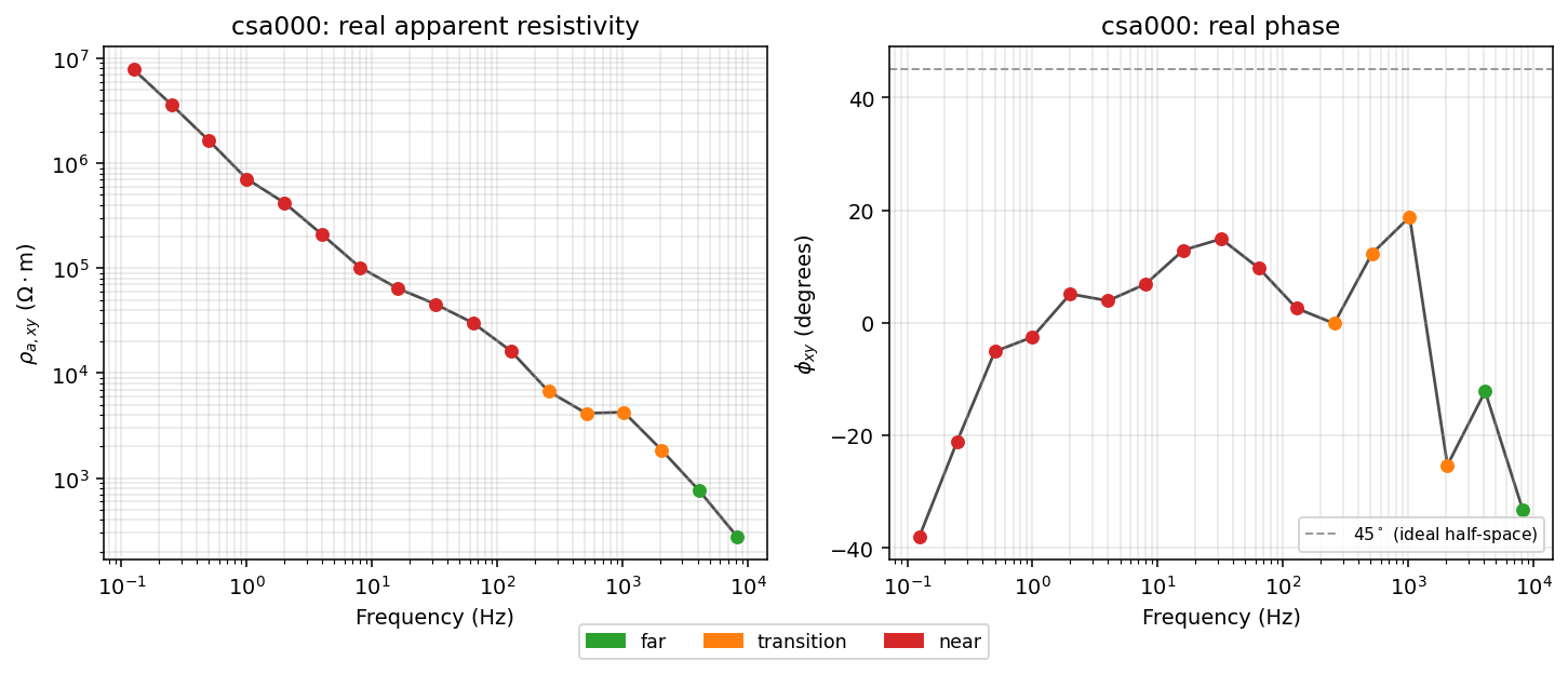
Left: the near-field points (red) trace a nearly straight power-law rise, exactly (2)’s regime where the geometric near-field term dominates over induction. Right: phase never gets close to the ideal \(45^\circ\) half-space value even at the two far-field points – a reminder that field-zone classification flags one specific distortion mechanism, not every reason a sounding looks imperfect (Static Shift and near-surface heterogeneity are independent, additional explanations).#
5.3. Classifying Field Zones Across A Profile#
The same classification, run over all ten stations at once and plotted as
a period-versus-station pseudosection with
pycsamt.emtools.fieldzone.plot_field_zones(), shows the near field
setting in earlier (at higher frequency, shorter period) almost everywhere
along the line, with a slightly more resistive patch around stations
csa150-csa200 pushing the far/transition boundary out to a longer
period:
>>> from pycsamt.emtools.fieldzone import plot_field_zones
>>> ax = plot_field_zones(sites, source_offset=1000.0, sort_by="name")
>>> ax.get_title()
'CSAMT Field Zone Classification (|k·r|)'
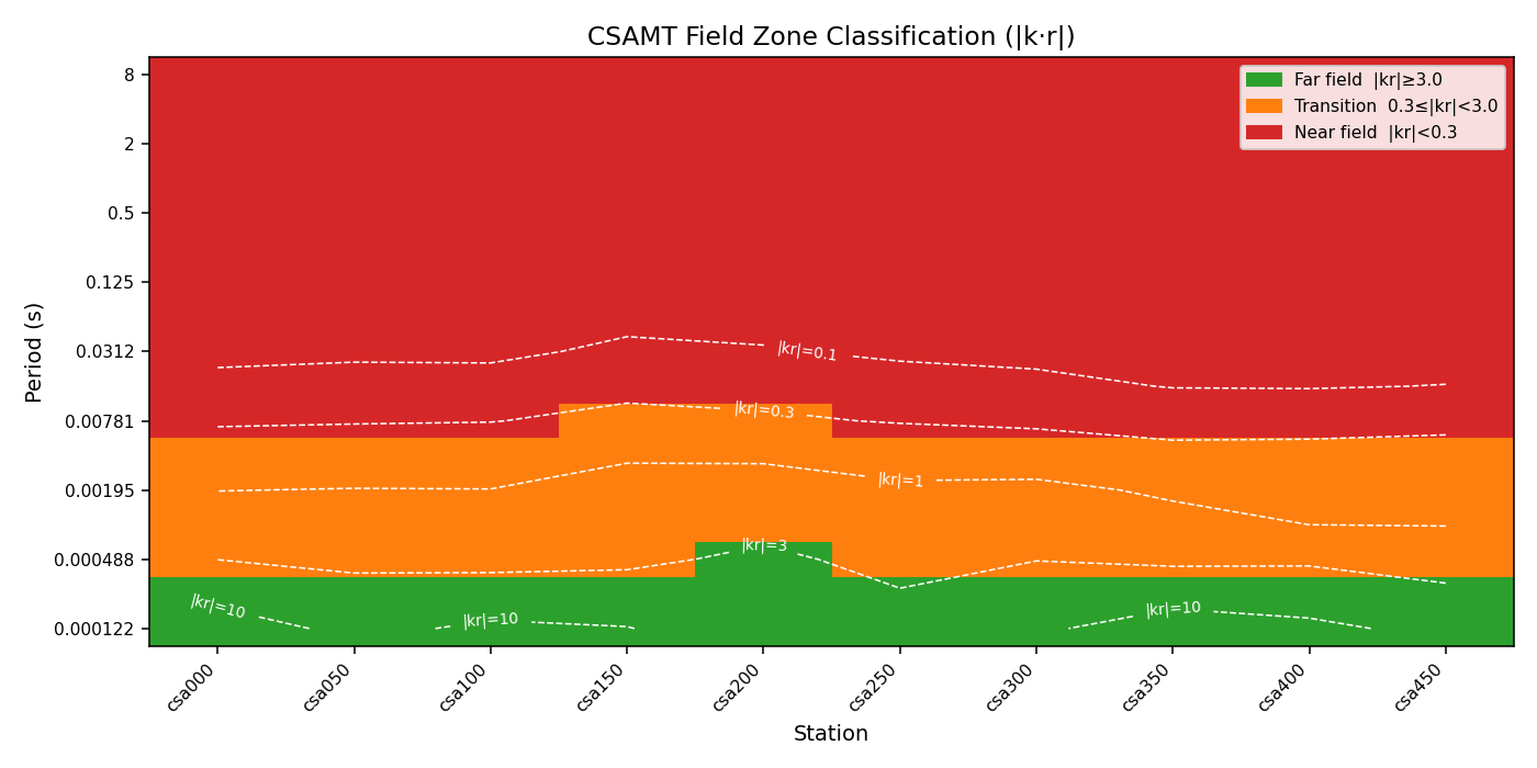
Dashed contours are constant \(|k\cdot r|\). The far-field (green) band stays below about 0.0005 s of period at every station – meaning, at this assumed 1 km offset, only the top one or two frequencies of the whole 17-frequency comb are trustworthy for a direct plane-wave interpretation.#
5.4. The Near-Field Correction Factor#
Rather than only flagging the problem, Chen & Yan (2005) give an analytical correction. For the equatorial electric field of a horizontal electric dipole over a homogeneous half-space, the ratio of the true field to its far-field (plane-wave) approximation is
\(F(p)\to1\) in the far field; \(|F(p)|^2\) is the multiplicative
bias on apparent resistivity introduced by the near-field geometry.
pycsamt.emtools.fieldzone.near_field_factor() evaluates
(3) per frequency:
>>> from pycsamt.emtools.fieldzone import near_field_factor
>>> nff = near_field_factor(sites, source_offset=1000.0)
>>> n0 = nff[nff["station"] == "csa000"].reset_index(drop=True)
>>> n0.loc[[0, 3, 8, 16], ["freq_hz", "nf_factor"]].round(4)
      freq_hz     nf_factor
0   8196.7220  9.995000e-01
3   1023.5410  7.920000e-01
8     32.0513  6.860911e+03
16     0.1250  6.714857e+10
At 8196.7 Hz, \(|F(p)|\approx1\) – the far-field approximation is essentially exact, matching the “far” label above. By 32 Hz it has grown to nearly 7000, and by the lowest frequency to \(6.7\times10^{10}\): the geometric near-field term does not just bias the data a little, it overwhelms it completely at this offset.
5.5. Applying – And Trusting – A Correction#
pycsamt.emtools.source_effects.correct_near_field() divides the
observed impedance by \(F(p)\) per frequency,
\(\mathbf{Z}_{\mathrm{corrected}}=\mathbf{Z}_{\mathrm{obs}}/F(p)\), to
recover a plane-wave-equivalent impedance:
>>> from pycsamt.emtools.source_effects import correct_near_field
>>> corrected = correct_near_field(sites, source_offset=1000.0, inplace=False)
>>> raw, cor = sites[0], corrected[0]
>>> ratio = cor.rho[:, 0, 1] / raw.Z.res_xy
>>> np.round(ratio[[0, 1, 2, 3, 4]], 4)
array([1.001 , 1.0113, 1.0979, 1.594 , 0.4571])
>>> np.round(ratio[[8, 12, 16]], 6)
array([0., 0., 0.])
In the far and transition zone (the first five entries, 8196.7-512.8 Hz), the correction is a modest, plausible adjustment – exactly what an analytical bias correction should look like. Below that, the “corrected” resistivity is not a smaller version of the near-field bias; it is numerically zero, because dividing a finite impedance by \(|F(p)|\sim10^4\)-\(10^{10}\) (as just measured above) drives the ratio below floating-point resolution. This is not a bug in the correction: (3) is doing exactly what its own asymptotic form says as \(p\to0\). It is a real limit on what an analytical near-field correction can do – it removes a mild geometric bias in the transition zone; it cannot resurrect deep near-field data where the geometric term has completely overwhelmed the induction signal. The practical conclusion is the same one Static Shift reaches about correcting frequency-dependent distortion with one scalar factor: know the difference between “correctable bias” and “data that should be masked”, and do not apply the formula past where it stops meaning anything.
5.6. Source Overprint And The Shadow Effect#
Yan & Fu (2004) frame the same physics as a source overprint question: is the ground-wave term big enough, relative to the surface-wave term, to distort a sounding? Their \(\beta\) ratio does exactly that, and does not require reducing the whole tensor to a single dimensionless number the way \(|k\cdot r|\) does – it is evaluated directly from \(\rho\), \(f\), and \(r\):
>>> from pycsamt.emtools.source_effects import overprint_beta
>>> beta = overprint_beta(sites[0].Z.res_xy, sites[0].Z.freq, 1000.0)
>>> np.round(beta[[0, 1, 2, 8]], 4)
array([1.62000e-02, 3.56620e+00, 2.30538e+01, 4.99954e+01])
At the highest frequency \(\beta=0.016\%\), far below the 3% threshold
Yan & Fu propose – clean data. One step down in frequency it is already
3.57%, just over the line, and by the third frequency it has jumped to
23%, saturating near 50% for the rest of the comb.
detect_source_overprint() packages
this as a per-frequency flag:
>>> from pycsamt.emtools.source_effects import detect_source_overprint
>>> det = detect_source_overprint(sites, source_offset=1000.0, beta_threshold=3.0)
>>> d0 = det[det["station"] == "csa000"]
>>> int(d0["overprint_flag"].sum()), len(d0)
(16, 17)
Sixteen of seventeen frequencies are flagged – consistent with the near-field picture above, since \(\beta\) and \(|k\cdot r|\) are two views of the same underlying physics.
A second, complementary diagnostic from Da et al. (2016) needs no offset
at all: it looks only at the shape of the sounding, comparing the
log-log slope of \(\rho_a\) versus frequency below and above a split
frequency. A strongly negative slope_delta (low-frequency slope much
steeper than high-frequency slope) points to the same resistivity
contrast beneath the source that produces the overprint:
>>> from pycsamt.emtools.source_effects import source_overprint_table
>>> tbl = source_overprint_table(sites, source_offset=None, f_split=1.0)
>>> row = tbl[tbl["station"] == "csa000"].iloc[0]
>>> round(row["lf_slope"], 3), round(row["hf_slope"], 3), round(row["slope_delta"], 3)
(-1.129, -0.813, -0.316)
source_offset=None here is deliberate, not an oversight: the
low/high-frequency slope columns are computed purely from the observed
\(\rho_a(f)\) curve and need no assumed geometry, unlike every other
diagnostic on this page. That makes them the one result here that is not
contingent on the illustrative 1 km offset – useful when a real offset
genuinely is not known.
5.7. A Second Convention: Wang & Lin (2023)#
Not every published field-zone criterion uses Bostick depth.
pycsamt.emtools.source_effects.normalize_response() implements Wang
& Lin (2023)’s version, built on the plain skin depth already labelled as
(8) in CSAMT, AMT, and MT Overview
(\(\delta\approx503\sqrt{\rho_a/f}\), not the 0.71x-smaller Bostick
depth), with different zone thresholds (0.5 and 4.0 rather than 0.3 and
3.0):
>>> from pycsamt.emtools.source_effects import normalize_response
>>> wl = normalize_response(sites, rho_ref=1000.0, source_offset=1000.0, comp="xy")
>>> w0 = wl[wl["station"] == "csa000"].reset_index(drop=True)
>>> w0["zone"].value_counts().to_dict()
{'near': 12, 'transition': 3, 'far': 2}
Twelve near-field points here versus eleven for the Bostick-based
classify_field_zones() earlier – close,
but not identical, because a different depth formula and different
thresholds move the transition/near boundary from 128 Hz to 255.8 Hz for
this station. Neither number is “more correct”; they are two different
published conventions, and a report should always state which one
produced a given zone label rather than quoting “near field” as if it
were convention-free.
5.8. Field Zones In Other Methods#
Everything above is specific to a fixed, known transmitter position, which is what makes CSAMT’s near/transition/far distinction meaningful in the first place:
MT and AMT have no controlled transmitter to be close to or far from. Their natural source is treated as a plane-wave field by assumption at essentially all usual survey scales, so the near/far dichotomy on this page does not apply – the corresponding caution in natural-source work is Static Shift and 3-D distortion, not source geometry.
TDEM has its own diffusion-based depth scale, \(z(t)\propto\sqrt{\rho t/\mu_0}\) (labelled (1) in TDEM Basics), and its own “how far into the approximation can I trust this gate” question – but the transmitter is switched off before the measurement is made, so there is no steady-state ground-wave/surface-wave split to speak of. The two pages’ depth formulas share the same square-root-of-resistivity-over-frequency shape for a genuinely different physical reason: one is a spatial near/far-field geometry effect at fixed frequency, the other is a time-domain diffusion depth.
5.9. Practical Guidance#
Before trusting a CSAMT sounding as plane-wave data:
Confirm the transmitter-receiver offset was actually recorded – pyCSAMT’s own EDI files here did not carry it, and every diagnostic on this page is only as good as that number.
Compute \(|k\cdot r|\) or \(\beta\) per frequency rather than assuming one zone applies to a whole sounding; the Tongkeng example above spans far, transition, and near field within one 17-frequency comb.
Prefer the shape-based slope diagnostic (
source_overprint_table()) when the offset is uncertain or unavailable.Treat
correct_near_field()as a bias correction for the transition zone, not a way to rescue deep near-field frequencies – mask those instead.State which convention (Chen & Yan / Bostick depth, or Wang & Lin / skin depth) produced a reported zone label.
5.10. Common Pitfalls#
assuming a station is “far field” because most of its frequencies are, when the low-frequency end (often the geologically interesting end) is actually near field;
running a correction formula outside its valid range and reporting the numerically-collapsed result as real data;
comparing \(|k\cdot r|\) values computed with different depth conventions as if they were the same number;
treating field-zone classification as a complete explanation for a poor sounding, when static shift or 3-D structure may also be present;
forgetting to record the transmitter-receiver offset in the field notebook, since no bundled or standard EDI field carries it.
5.11. Next Steps#
Continue with:
CSAMT, AMT, and MT Overview for the method-family context this page extends;
Impedance Tensor for the plane-wave tensor formalism these corrections restore;
Static Shift for the other major amplitude-only CSAMT/MT distortion;
TDEM Basics for the time-domain analogue of the depth-scale idea.
5.12. References#
The field-zone parameter, near-field correction factor, and shadow-effect
analysis follow [Chen2005] and [Yan2004]. The shape-based slope
diagnostic follows [Da2016]. The alternative skin-depth-based convention
follows [WangLin2023]. The bundled CSAMT survey used throughout this page
is published in [Kouadio2020] – see data/CSAMT/README.md for the
full station table and citation.