6.3.6. Solver-neutral Maxwell contracts

Architecture roadmap’s governing equation (2) can be solved by more than one program: an in-repo finite-difference solver, a research-only in-house 3-D curl-curl solve, or an external Fortran executable. Every one of those needs to hand Loss functions for scientific inversion and Recovery, residual, and OOD diagnostics the same shape of answer, or those packages would need a special case per solver. pycsamt.forward.maxwell is that shared boundary: a problem/result contract every backend consumes and produces identically, a validated execution path no adapter can bypass, and a set of analytic benchmarks that turn “this backend works” from a claim into a number.

6.3.6.1. The problem and result contracts

A MaxwellMesh is a rectilinear grid of cell edges; a ReceiverSet is named observation locations in that mesh’s coordinates. Together with a conductivity array and a frequency list, they make up a MaxwellProblem — every physical input a backend needs and nothing else:

>>> import numpy as np
>>> from pycsamt.forward.maxwell import (
...     MaxwellMesh, ReceiverSet, MaxwellProblem,
... )

>>> mesh = MaxwellMesh(np.linspace(0, 10_000, 41), np.linspace(0, 5_000, 31))
>>> mesh.shape, mesh.dimension
((30, 40), 2)
>>> receivers = ReceiverSet([[5_000.0, 0.0]], ["S00"])
>>> problem = MaxwellProblem(
...     mesh,
...     np.full(mesh.shape, 1.0 / 100.0),
...     [10.0, 1.0],
...     receivers,
...     ("zxy", "zyx"),
... )
>>> problem.problem_hash
'0db2d50b944706f3ad5f349e3d5c71e9d3c182bf5357373f0f7fa2788301308a'

That hash is deterministic in the physical content, not the Python object identity: building the exact same mesh, conductivity, frequencies, and receivers a second time reproduces it exactly, which is what lets cache key a cache entry, or an experiment record pin the problem it was tested against, by content rather than by an incidental variable name. The contract also rejects a request the physics cannot honor, before any solver ever sees it:

>>> MaxwellProblem(
...     mesh, np.full(mesh.shape, 0.01), [10.0], receivers, ("zxx",)
... )
Traceback (most recent call last):
...
ValueError: 2-D problems support only zxy and zyx impedance components.

A 2-D TE/TM formulation has no zxx/zyy diagonal response by construction, so requesting one is not a solver limitation to work around — it is a request the 2-D physics itself cannot answer, and MaxwellProblem says so immediately rather than letting a solver silently return zeros for it. ForwardResult is the matching output half of the contract: complex impedance in the same canonical (station, frequency, component) order SurveyData uses, plus a SolverDiagnostics record of convergence and residuals — never a bare array a caller has to trust blindly.

The contract stores SI impedance in volts per ampere. For angular frequency \(\omega=2\pi f\) and magnetic permeability \(\mu\), the observable quantities normally inspected by an MT user, apparent resistivity and phase, are

(1)\[\rho_a(f)=\frac{|Z(f)|^2}{\omega\mu}, \qquad \phi(f)=\operatorname{atan2}(\Im Z(f),\Re Z(f)).\]

Equation (1) is also an immediate unit check: substituting EDI field units directly would produce the wrong apparent resistivity scale. Under the package’s exp(+iwt) convention, the analytic zxy half-space response has positive 45-degree phase:

>>> import numpy as np
>>> from pycsamt.forward.maxwell.benchmarks import half_space_impedance

>>> frequency = np.array([100.0, 10.0, 1.0, 0.1])
>>> impedance = half_space_impedance(100.0, frequency)
>>> np.round(impedance, 6)
array([0.198692+0.198692j, 0.062832+0.062832j,
       0.019869+0.019869j, 0.006283+0.006283j])
>>> mu0 = 4e-7 * np.pi
>>> rho_a = np.abs(impedance) ** 2 / (2 * np.pi * frequency * mu0)
>>> np.round(rho_a, 6)
array([100., 100., 100., 100.])
>>> np.round(np.angle(impedance, deg=True), 3)
array([45., 45., 45., 45.])

Do not infer a component convention from phase alone. Reversing electric or magnetic field orientation changes an impedance sign and can shift the raw phase by 180 degrees without changing \(\rho_a\). Compare components only after matching axis orientation, Fourier convention, and any phase wrapping; the canonical names preserve order, but they cannot repair incompatible input conventions.

6.3.6.2. A validated execution path, not just an interface

Any Python object with a matching solve method could call itself a Maxwell backend; nothing would stop it from returning a result with the wrong axes or silently claiming success on a diverged solve. That is exactly what BaseMaxwellAdapter closes off: every adapter’s solve() assesses the problem against declared BackendCapabilities first, runs the concrete backend second, and validates the returned result against the problem a third time — a subclass only ever implements the middle step, so it cannot skip the checks around it even by accident. The two demonstration adapters below make each check concrete instead of abstract:

>>> from pycsamt.forward.maxwell import (
...     SolverDiagnostics, ForwardResult, BackendCapabilities,
...     CallableMaxwellAdapter,
... )

>>> cap_3d_only = BackendCapabilities(
...     "demo3d", "1", (3,), ("zxy", "zyx"), verified_benchmarks=("half-space",)
... )
>>> def solver_ok(p):
...     diagnostics = SolverDiagnostics([[True]], [[0]], [[0.0]], 0.01)
...     return ForwardResult(
...         p.problem_hash, p.frequencies_hz, p.receivers.names,
...         p.components, [[[1 + 1j]]], None, "demo3d", "1", diagnostics,
...     )
>>> CallableMaxwellAdapter(cap_3d_only, solver_ok).solve(problem)
Traceback (most recent call last):
...
pycsamt.forward.maxwell.adapters.IncompatibleProblemError: backend 'demo3d' is incompatible: 2-D problems are unsupported

The 3-D-only adapter never even calls its solver: capability assessment rejects the 2-D problem first. A backend that declares the right dimension can still fail the third check, by returning something that does not match what was actually asked for:

>>> cap_2d = BackendCapabilities(
...     "demo2d", "1", (2,), ("zxy", "zyx"), verified_benchmarks=("half-space",)
... )
>>> def solver_wrong_axes(p):
...     diagnostics = SolverDiagnostics(
...         [[True], [True]], [[0], [0]], [[0.0], [0.0]], 0.01
...     )
...     return ForwardResult(
...         p.problem_hash, p.frequencies_hz, p.receivers.names,
...         ("zyx",), [[[1 + 1j], [1 + 1j]]], None, "demo2d", "1", diagnostics,
...     )
>>> CallableMaxwellAdapter(cap_2d, solver_wrong_axes).solve(problem)
Traceback (most recent call last):
...
pycsamt.forward.maxwell.adapters.InvalidBackendResultError: result frequency, receiver, or component axes do not match the problem.

Here the solver ran, but returned zyx when the problem asked for zxy/zyx together — a mistake that would silently corrupt a downstream array shape if nothing were checking for it. AdapterPolicy controls the rest of that third check: whether every solve must have converged, whether a maximum relative residual is enforced, and whether an ordinary Python exception raised inside a backend is wrapped into a BackendExecutionError (the default) or left to propagate as-is.

6.3.6.3. Meshes built from geology, not by hand

Writing mesh edges by hand, as the minimal examples above do, does not scale to a real earth model that needs padding or may carry a topographic surface. build_solver_mesh() takes a GeologyGrid and returns a padded, air-layered SolverMeshModel ready to become a problem:

>>> from pycsamt.ai.geology import GeologyGrid
>>> from pycsamt.forward.maxwell import MeshDesign, build_solver_mesh

>>> grid = GeologyGrid.regular_2d(nx=20, nz=12, dx_m=200, dz_m=100)
>>> model = build_solver_mesh(
...     grid,
...     resistivity_ohm_m=np.full(grid.shape, 100.0),
...     frequencies_hz=[10.0, 1.0],
...     design=MeshDesign(
...         horizontal_padding_cells=6,
...         bottom_padding_cells=8,
...         air_layers=8,
...     ),
... )
>>> model.mesh.shape
(28, 32)
>>> model.core_slices
(slice(8, 20, None), slice(6, 26, None))
>>> model.quality.acceptable, model.quality.cell_count
(True, 896)

core_slices is exactly where the original 12x20 geological grid sits inside the padded 28x32 solver mesh — the difference is eight air layers on top, eight padding cells below, and six on each side, each grown geometrically rather than added at core resolution, which would waste cells far from the region anyone cares about. acceptable reports whether that padding is actually adequate, using the same skin depth already defined in equation (12): skin_depth_m() computes it exactly rather than through that equation’s decimal approximation, and cells_per_minimum_skin_depth checks the core mesh actually resolves it:

>>> from pycsamt.forward.maxwell import skin_depth_m
>>> round(float(skin_depth_m(100, 1)), 1)
5032.9
>>> round(model.quality.cells_per_minimum_skin_depth, 2)
7.96

Roughly eight core cells span the largest skin depth this problem’s frequencies produce, above the default four-cells-per-skin-depth target, so model.quality.warnings is empty. Before handing the model to a solver, assess_receivers() checks that every receiver actually falls inside the mesh and on or above the local terrain — a cheap geometric check worth running before a much more expensive solve fails on the same problem:

>>> receivers = ReceiverSet(
...     [[float(x), 0.0] for x in grid.x_m[::4]],
...     [f"S{i:02d}" for i in range(len(grid.x_m[::4]))],
... )
>>> model.assess_receivers(receivers)
()
>>> problem_from_model = model.to_problem(
...     [10.0, 1.0], receivers, components=("zxy", "zyx")
... )
>>> problem_from_model.mesh.shape, problem_from_model.receivers.count
((28, 32), 5)

An empty tuple from assess_receivers means no error was found; to_problem() would have raised on exactly the same check if a receiver had been placed below the surface or outside the padded mesh.

build_solver_mesh is a geometry builder, not a promise that every backend can use every geometry it represents. Its air mask and terrain surface can be preserved for a future capable adapter, but MT2DAdapter, MT3DAdapter, and the current v1 ModEm3DAdapter all declare supports_inactive_cells=False and supports_topography=False. Passing mark_air_inactive=True to to_problem is therefore incompatible with those adapters, and treating air cells as conductive does not become physical topography. Always call adapter.assess(problem) after mesh construction; an empty receiver-geometry report alone checks locations, not backend physics.

Padding enough is not automatic, and neither is knowing which boundary controls the error. The executed width study below holds the vertical mesh fixed and changes the lateral extent from 20 to 240 km. For a uniform half-space the four curves nearly coincide: the adapter supplies the exact 1-D edge-column boundary response, and there is no lateral conductivity gradient for a side boundary to truncate. The growing high-frequency error is instead shared by every width and follows the fixed near-surface vertical resolution becoming coarse relative to the shrinking skin depth.

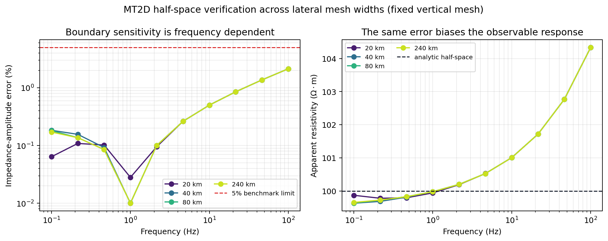
An executed MT2D mesh sensitivity study with an identical vertical mesh. Overlapping width curves rule out lateral extent as the dominant error in this controlled half-space case.

The result must not be generalized into “width never matters.” A laterally uniform analytic benchmark cannot exercise reflections or truncation caused by a 2-D conductivity contrast near a side boundary. For heterogeneous models, repeat the solve after independently enlarging lateral padding, bottom padding, and near-surface resolution, and require the response change to fall below a declared tolerance. MeshQuality.acceptable is an advisory geometric gate; mesh convergence of the requested observables is the numerical evidence.

6.3.6.4. Proven against physics, not asserted

A backend that runs without raising is not the same as a backend that computes correct impedance. benchmarks exists to close that gap with analytic references a real solver has no way to satisfy by accident. For a uniform half-space of resistivity \(\rho\), the analytic surface impedance is

(2)\[Z(\omega) = \sqrt{i\,\omega\,\mu_0\,\rho},\]

and for a stack of layers it follows from recursing equation (2)’s intrinsic impedance upward through each interface, starting from the basal half-space \(Z_N = \sqrt{i\omega\mu_0\rho_N}\) and, for each layer \(\ell\) from \(N-1\) down to \(1\) with intrinsic impedance \(\zeta_\ell=\sqrt{i\omega\mu_0\rho_\ell}\), wavenumber \(k_\ell=\sqrt{i\omega\mu_0/\rho_\ell}\), and thickness \(h_\ell\), applying

(3)\[Z_\ell = \zeta_\ell\, \frac{Z_{\ell+1} + \zeta_\ell\tanh(k_\ell h_\ell)} {\zeta_\ell + Z_{\ell+1}\tanh(k_\ell h_\ell)}.\]

half_space_impedance() and layered_earth_impedance() implement equations (2) and (3) directly, and half_space_benchmark()/ layered_earth_benchmark() package them into a MaxwellBenchmark that any conforming adapter can run against. Against the mesh calibrated above, MT2DAdapter genuinely passes both:

For valid predicted and reference values \(Z_i\) and \(Z_i^{\mathrm{ref}}\), the benchmark reports three complementary errors,

(4)\[\begin{split}\begin{aligned} E_{\mathrm{NRMS}} &= \sqrt{\frac{\sum_i|Z_i-Z_i^{\mathrm{ref}}|^2} {\sum_i|Z_i^{\mathrm{ref}}|^2}},\\ E_A &= \max_i \frac{\bigl||Z_i|-|Z_i^{\mathrm{ref}}|\bigr|} {|Z_i^{\mathrm{ref}}|},\\ E_\phi &= \max_i \left|\arg\!\left(\frac{Z_i}{Z_i^{\mathrm{ref}}}\right)\right|. \end{aligned}\end{split}\]

The ratio inside \(E_\phi\) gives a circular phase difference, avoiding a false 358-degree error across the \(-180/180\) branch cut. Default limits are 0.05 for \(E_{\mathrm{NRMS}}\), 0.05 for \(E_A\), 2 degrees for \(E_\phi\), complete validity, and successful solver diagnostics. Passing only one of these checks is not a benchmark pass.

>>> from pycsamt.forward.maxwell.benchmarks import (
...     half_space_benchmark, layered_earth_benchmark,
... )
>>> from pycsamt.forward.maxwell.mt2d import MT2DAdapter

>>> dz = 25.0 * 1.22 ** np.arange(34)
>>> z_edges = np.concatenate([[0.0], np.cumsum(dz)])
>>> calibrated_mesh = MaxwellMesh(np.linspace(0, 240_000, 25), z_edges)
>>> station = ReceiverSet([[120_000.0, 0.0]], ["S00"])
>>> adapter = MT2DAdapter(verbose=False)

>>> half_space = half_space_benchmark(
...     calibrated_mesh, station, [10.0, 1.0], resistivity_ohm_m=100.0
... )
>>> outcome = half_space.run(adapter)
>>> outcome.passed
True
>>> round(outcome.metrics.normalized_rms, 5)
0.00862

>>> interface1, interface2 = z_edges[8], z_edges[16]
>>> layered = layered_earth_benchmark(
...     calibrated_mesh, station, np.logspace(-1, 1, 6),
...     [100.0, 30.0, 500.0], [interface1, interface2 - interface1],
... )
>>> layered.run(adapter).passed
True

The same API preserves a failed outcome and explains every violated limit. Using the earlier shallow 10-by-5 km mesh across 10 to 0.1 Hz gives:

>>> shallow = half_space_benchmark(
...     mesh, ReceiverSet([[5_000.0, 0.0]], ["S00"]),
...     [10.0, 1.0, 0.1], resistivity_ohm_m=100.0,
... )
>>> failed = shallow.run(adapter)
>>> failed.passed
False
>>> (round(failed.metrics.normalized_rms, 4),
...  round(failed.metrics.maximum_amplitude_relative_error, 4),
...  round(failed.metrics.maximum_phase_error_deg, 3))
(0.0707, 0.0538, 2.997)
>>> failed.failures
('normalized RMS 0.0706959 exceeds 0.05',
 'maximum amplitude relative error 0.0538247 exceeds 0.05',
 'maximum phase error 2.99718 deg exceeds 2 deg')

This is useful evidence, not an exception to suppress: all values are finite and the solver ran, yet the discretized problem is not accurate enough for the declared scientific tolerance.

A 0.86% normalized RMS error, well inside the default 5% threshold, is MT2DAdapter’s genuine accuracy on this mesh over the 0.1-10 Hz band the benchmark actually tests — not a rounded claim.

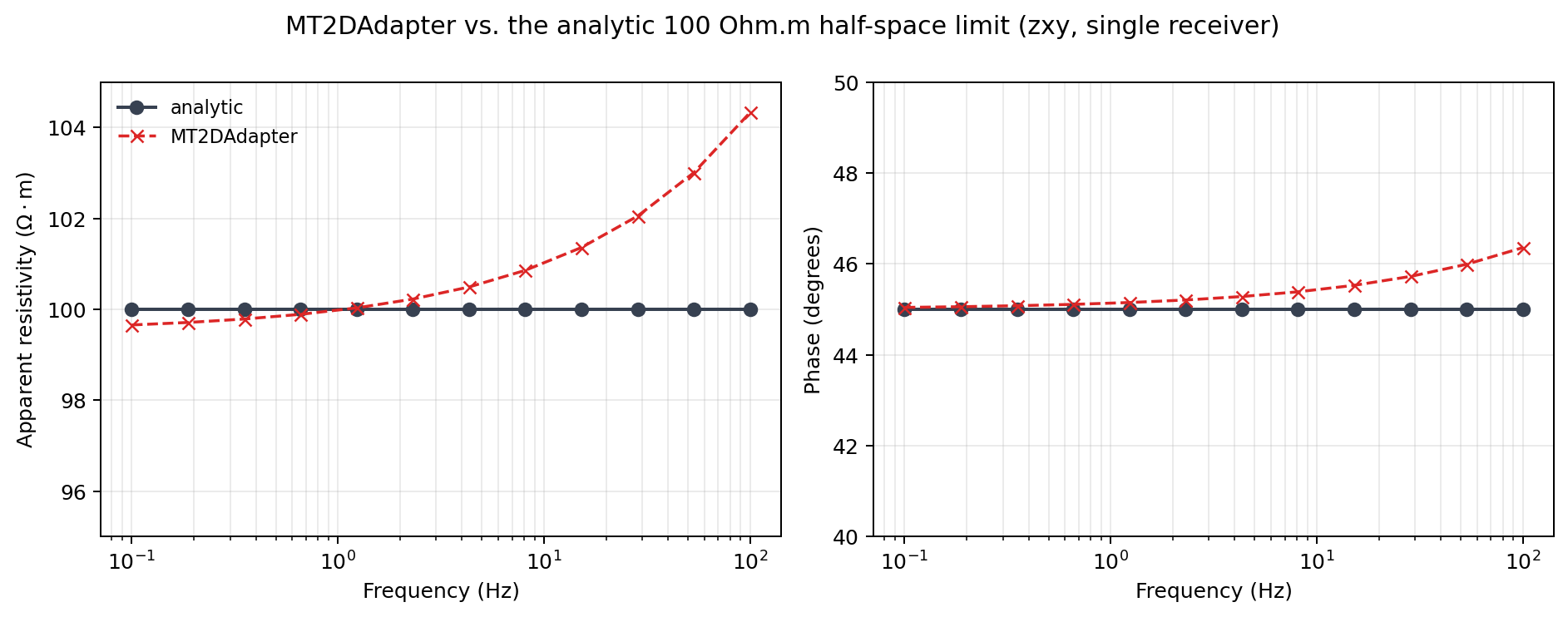
Extending the same mesh and adapter to 100 Hz, well past the 0.1-10 Hz band the benchmark above validates, shows agreement degrading toward the highest frequencies: a smaller skin depth there is resolved by relatively fewer cells on a mesh whose near-surface resolution was calibrated for the lower, benchmarked band. This is exactly the risk equation (12) and this page’s mesh-quality checks exist to catch — a solver’s validated accuracy is a property of one mesh and one frequency band, not a permanent property of the adapter.

6.3.6.5. What the solved 3-D backends guarantee

Both 3-D adapters now solve the frequency-domain curl–curl system, under the package’s exp(+iwt) convention,

(5)\[\nabla\times\nabla\times\mathbf E +i\omega\mu_0\sigma\mathbf E=\mathbf 0, \qquad \mathbf H=-\frac{\nabla\times\mathbf E}{i\omega\mu_0}.\]

MT3DAdapter discretizes equation (5) on a staggered Yee grid. Electric fields live on edges, magnetic fields on faces, and the non-uniform curl uses dual-grid distances. This detail is essential: on a graded mesh the dual distance between neighbouring faces is not either cell’s individual width. Two horizontal source polarizations are solved at each frequency and combined at each receiver to recover zxx, zxy, zyx, and zyy.

The pure-Python adapter is still research-only because it uses a direct sparse solve and rejects more than 6,000 cells by default. Non-uniform support solves the earlier mesh-design failure: a fine geological core can now be padded to several skin depths without paying for fine cells throughout the domain. It does not make direct factorization scale to a production survey. On the calibrated 4,096-cell mesh it passes both analytic gates at 0.5–2 Hz: about 1.9% normalized RMS for the half-space and about 3.5% for the layered earth. Those numbers validate that mesh and band, not arbitrary tens-of-hertz grids.

ModEm3DAdapter maps the same MaxwellProblem to the compiled ModEM Mod3DMT forward executable and converts its native field impedance back to SI V/A. The adapter shifts stations and model cells together into ModEM-local coordinates, always asks ModEM for the full tensor, and then filters the returned components into the caller’s requested order. A real compiled v6.2.6 binary passes the half-space and layered-earth gates below 5% normalized RMS on the tested 8x8x10, 300 m-cell mesh at 0.5–1 Hz.

The following output was executed directly from the current capability objects:

>>> from pycsamt.forward.maxwell.mt3d import MT3DAdapter
>>> from pycsamt.forward.maxwell.modem3d import ModEm3DAdapter

>>> for backend in (MT3DAdapter(), ModEm3DAdapter()):
...     cap = backend.capabilities
...     print(cap.name, cap.version)
...     print(cap.dimensions, cap.components)
...     print(
...         cap.supports_nonuniform_mesh,
...         cap.supports_topography,
...         cap.supports_inactive_cells,
...         cap.supports_anisotropy,
...     )
...     print(cap.maximum_cells, cap.verified_benchmarks)
mt3d 1.0-research
(3,) ('zxx', 'zxy', 'zyx', 'zyy')
True False False False
6000 ('half-space', 'layered-earth')
modem3d modem-v6.2.6-adapter-1.0
(3,) ('zxx', 'zxy', 'zyx', 'zyy')
True False False False
None ('half-space', 'layered-earth')

The shared capability list should not hide their different diagnostics. MT3DAdapter reports a measured algebraic residual from its sparse solve. ModEM’s predicted-data file exposes neither an iterative residual nor an iteration history, so the v1 adapter stores finite placeholders of 0.0 and zero iterations while reporting real wall-clock time. A ModEM residual of zero is therefore not evidence of an exact linear solve; analytic and mesh-refinement comparisons remain the accuracy evidence.

Both adapters enforce surface receivers, horizontal containment, isotropic conductivity, vacuum permeability, and no inactive cells or terrain. ModEM additionally requires the top mesh edge at \(z=0\) and at least ten earth cells in depth, because its internal ten-air-layer setup otherwise reads past the available earth widths. These are adapter-v1 restrictions and preflight checks; they must not be generalized into claims about everything the ModEM solver itself can represent.

6.3.6.6. Backends found by capability, not by import

A caller building a training dataset should not need to know which Python module implements "mt2d". assess answers the compatibility question directly from an adapter’s own declared capabilities, without running the solver at all:

>>> report = adapter.assess(problem_from_model)
>>> report.compatible, report.errors
(True, ())
>>> adapter.capabilities.verified_benchmarks
('half-space', 'layered-earth')

Architecture roadmap shows the process-wide backend registry this capability declaration feeds — looking up "mt2d" or "modem3d" by name and inspecting what each one honestly claims — rather than repeating that example here.

6.3.6.7. Caching and batch generation

A single solve above finishes in well under a second; a training dataset needs thousands of them, and a run that is interrupted partway through should not have to start over. MaxwellResultCache is a content-addressed, multi-process-safe cache keyed by problem_hash, so the same problem is never solved twice across separate calls, processes, or restarts:

>>> from pathlib import Path
>>> from tempfile import TemporaryDirectory
>>> from pycsamt.forward.maxwell import MaxwellResultCache

>>> with TemporaryDirectory() as directory:
...     cache = MaxwellResultCache(directory)
...     print(cache.contains(problem))
...     first = cache.get_or_solve(problem, adapter)
...     second = cache.get_or_solve(problem, adapter)
...     print(cache.contains(problem))
False
True

The second call above reused the first call’s stored, checksum-verified archive instead of invoking the solver again — the point is not raw speed on one small problem, but that regenerating the same dataset twice, or resuming after a crash partway through, never silently redoes work or drifts from what was already computed.

The cache key is the problem_hash; it does not include backend name, backend version, adapter policy, or software revision. The stored ForwardResult retains its backend identity and is checksum-verified, but get_or_solve(problem, another_adapter) can still return the existing result because the physical problem key matches. Use a separate cache root per backend/version when comparing solvers, and record both the problem hash and the returned backend identity. Cache integrity means the archived result was not corrupted; it does not mean every backend would produce the same result.

solve_batch() builds on this cache to solve many problems at once, retrying only the exceptions a BatchPolicy marks transient and collecting every terminal failure into a FailureManifest instead of aborting the whole run — exactly the machinery 2-D Maxwell training-data generation and 3-D Maxwell training-data generation already show generating a real, versioned training dataset with it.