6.3.4. Correlated geological priors

Training a network on tiled 1-D models teaches it a per-station relationship, not a spatial one: nothing in that training data ever shows the network what a laterally continuous resistivity structure looks like. pycsamt.ai.geology exists to generate complete 2-D sections and 3-D volumes directly, so response simulation and training happen on a traceable geological prior instead of on independent columns stitched together after the fact.

The package builds on a shared GeologyGrid (canonical (z, x) or (z, y, x) cell-centre grid) and composes several generators on top of it: anisotropic correlated Gaussian fields (CorrelatedField, via generate_gaussian_field()), layered geology with dipping interfaces (generate_layered_geology()), ellipsoidal lenses and bodies (insert_lenses()), and topographic surfaces (TopographicSurface). Every generator takes an explicit random seed and exposes its generation provenance, so a training dataset can always be traced back to exactly the configuration that produced it.

The public objects are useful at different points in that construction. GeologyGrid fixes coordinates and canonical array order; GaussianCorrelation defines spatial scales; CorrelatedField and DirectionalVariogram carry sampled values and their diagnostics. LayeredGeology then exposes interfaces, named layer masks, resistivity, summaries, and persistence, while LensGeology adds named body masks, overlap diagnostics, and the chosen conflict policy. Finally, TopographicSurface keeps terrain sampling and the physics-facing earth mask aligned to the same grid. These are immutable result objects: create a new composition instead of editing their arrays in place.

>>> import numpy as np
>>> from pycsamt.ai.geology import GeologyGrid, GaussianCorrelation
>>> from pycsamt.ai.geology import generate_gaussian_field
>>> grid = GeologyGrid.regular_2d(nx=32, nz=16, dx_m=100, dz_m=50)
>>> model = GaussianCorrelation(length_x_m=500, length_z_m=100)
>>> field = generate_gaussian_field(grid, model, seed=12)
>>> field.values.shape
(16, 32)
>>> round(float(np.mean(field.values)), 6)
0.0
>>> round(float(np.std(field.values)), 6)
1.0

The field values are dimensionless standard-normal scores, not resistivity. They become geological parameters only after a caller assigns a distribution, for example through ElectricalLayer. Keeping that distinction explicit prevents a zero-centred Gaussian field from being passed to a forward solver as if negative conductivity were meaningful.

The returned field is more than its values array. field_hash identifies the values and provenance together, provenance() records the seed, correlation, boundary policy and grid, and rescale returns another immutable field with a requested sample mean and standard deviation:

>>> physical = field.rescale(mean=2.0, standard_deviation=0.25)
>>> round(float(physical.values.mean()), 6)
2.0
>>> round(float(physical.values.std()), 6)
0.25
>>> len(field.field_hash), field.provenance()["seed"]
(64, 12)

This rescaling still does not assign units. A mean of two could mean log10(ohm m), porosity, or another parameter; that semantic choice belongs in the dataset configuration and must travel with the array.

6.3.4.1. What a Gaussian correlation length means

In two dimensions the requested stationary covariance is

(1)\[C(h_x,h_z)=\exp\!\left[-\frac{1}{2} \left(\frac{h_x^2}{L_x^2}+\frac{h_z^2}{L_z^2}\right)\right].\]

Thus \(L_x\) and \(L_z\) are correlation length scales, not hard feature widths: at a one-length separation the correlation is \(e^{-1/2}\approx0.607\), and it approaches zero only asymptotically. The ratio \(L_x/L_z\) is exposed as anisotropy_xz. In 3-D, length_y_m supplies the second horizontal principal scale and azimuth_deg rotates the horizontal axes; azimuth has no role in 2-D.

The generator filters white noise in Fourier space with amplitude

(2)\[A(\mathbf k)=\exp\!\left[-\frac{1}{4} \left((k_xL_x)^2+(k_zL_z)^2\right)\right],\]

so the power multiplier \(|A|^2\) is the spectrum corresponding to equation (1). boundary="periodic" filters directly on the requested grid and therefore joins opposite edges. The default "reflect" filters a reflected doubled grid and crops its centre, reducing that artificial wrap-around. Neither policy makes a small domain representative: correlation lengths need several cells for numerical resolution and the domain needs several correlation lengths for statistical support. Extremely long lengths on a small grid are rejected when filtering produces a numerically constant field.

Standardization enforces the sample mean and population standard deviation of each realization to be exactly zero and one. This is convenient for consistent scaling but suppresses between-realization fluctuations in those two statistics. Set standardize=False when those fluctuations are part of the intended prior, or call rescale() when a precise sample mean and spread are required.

6.3.4.2. Verify correlation statistically

directional_variogram() computes the unbinned empirical variogram at integer cell lags,

(3)\[\widehat\gamma_a(m\Delta_a)=\frac{1}{2N_m} \sum_{(u,v)\in P_m}\left[g(v)-g(u)\right]^2,\]

where \(P_m\) contains pairs separated by \(m\) cells along axis \(a\) and \(N_m=|P_m|\). For a standardized Gaussian field, the theoretical curve is \(\gamma(h)=1-C(h)\), with a sill near one. Pair counts fall with lag, so the far end of a single realization’s variogram is the least stable part. This is why correlation recovery belongs at the ensemble level:

>>> from pycsamt.ai.geology import directional_variogram

>>> variogram_x = directional_variogram(field, "x", max_lag_cells=5)
>>> variogram_x.lag_m.tolist()
[100.0, 200.0, 300.0, 400.0, 500.0]
>>> variogram_x.pair_count.tolist()
[496, 480, 464, 448, 432]
>>> np.all(np.diff(variogram_x.pair_count) < 0)
True

The upper-right panel below aggregates 32 independently seeded fields. Once lag is divided by its requested directional length, the horizontal and vertical medians nearly collapse onto the theoretical Gaussian curve. The 10th–90th percentile envelopes remain broad, especially beyond two correlation lengths: one field cannot be expected to reproduce the population covariance exactly. The upper-left realization also shows the intended \(L_x/L_z>1\) texture as horizontally elongated patches rather than independent columns.

6.3.4.3. Build stratigraphy before adding bodies

ElectricalLayer defines a median resistivity and, optionally, correlated within-unit variability. Before clipping to declared bounds, the implemented model is

(4)\[\log_{10}\rho(\mathbf x)=\log_{10}\rho_{50}+s_{10}g(\mathbf x),\]

where \(\rho_{50}\) is resistivity_ohm_m, \(s_{10}\) is log10_std, and \(g\) is a standardized correlated field. Therefore resistivity_ohm_m is the lognormal median, not its arithmetic mean. A positive log10_std requires a correlation model; this prevents accidental cell-wise white-noise geology.

generate_layered_geology() generates correlated interface relief independently from within-layer heterogeneity. Interfaces are ordered from shallow to deep. minimum_thickness_m enforces separation; interface_policy="raise" rejects a crossing realization, while the default "project" moves infeasible surfaces into the allowed region and records the adjusted fraction. A large adjustment fraction means the proposed means, relief, and thickness are mutually inconsistent and should be revised, not quietly accepted as the intended prior.

>>> from pycsamt.ai.geology import ElectricalLayer
>>> from pycsamt.ai.geology import generate_layered_geology

>>> units = [
...     ElectricalLayer("cover", 20),
...     ElectricalLayer("sediments", 100),
...     ElectricalLayer("basement", 1000),
... ]
>>> layered = generate_layered_geology(
...     GeologyGrid.regular_2d(nx=24, nz=16, dx_m=100, dz_m=50),
...     units, [200, 500], seed=5,
...     interface_relief_std_m=[30, 50],
...     interface_correlation=GaussianCorrelation(600, 100),
... )
>>> layered.interface_depth_m.shape
(2, 24)
>>> summary = layered.summary()
>>> {name: round(value, 3) for name, value in summary["layer_fractions"].items()}
{'cover': 0.253, 'sediments': 0.37, 'basement': 0.378}
>>> round(summary["adjusted_interface_fraction"], 3)
0.0

The lower-left panel shows the result. White lines are continuous sampled interfaces; colour variation within the upper and lower units comes from separate correlated fields. Layer occupancy is worth recording across the whole dataset: a valid geometry can still be a poor training prior if a rare unit occupies too few cells or appears only at one depth.

6.3.4.4. Compose lenses with explicit overlap rules

An EllipsoidalLens uses the normalized rotated radius

(5)\[r(\mathbf x)=\sqrt{ \left(\frac{x'}{a_x}\right)^2+ \left(\frac{z'}{a_z}\right)^2},\]

in 2-D, with a corresponding \(y'\) term in 3-D. Cells with \(r\le1\) belong to the envelope. A non-zero transition_fraction applies a cubic smoothstep weight \(w\in[0,1]\) in the outer shell and blends in log resistivity,

(6)\[\log_{10}\rho_{\mathrm{new}}=(1-w)\log_{10}\rho_{\mathrm{base}} +w\log_{10}\rho_{\mathrm{lens}}.\]

Log-space blending preserves positivity and gives multiplicative rather than arithmetic transitions. When bodies overlap, declaration order is not allowed to decide silently: error, first, last, most_conductive, or most_resistive must state the rule.

>>> from pycsamt.ai.geology import EllipsoidalLens, insert_lenses

>>> lens = EllipsoidalLens(
...     "conductor", 1200, 350, 350, 100, 5,
...     transition_fraction=0.2,
... )
>>> composed = insert_lenses(layered, [lens], conflict_policy="error")
>>> lens_summary = composed.summary()
>>> round(lens_summary["assigned_fractions"]["conductor"], 4)
0.0521
>>> lens_summary["maximum_overlap"], lens_summary["conflict_policy"]
(1, 'error')
>>> round(float(np.min(composed.resistivity_ohm_m)), 3)
5.0

6.3.4.5. Topography is a mask, not a vertical stretch

interpolate_topography() and topography_from_sites() rasterize elevation onto the grid’s horizontal cell centres. With reference elevation \(e_0\), terrain depth and local cell depth are

(7)\[d_s(\mathbf x_h)=e_0-e(\mathbf x_h), \qquad d_{\mathrm{local}}(z,\mathbf x_h)=z-d_s(\mathbf x_h).\]

Cells with \(d_{\mathrm{local}}<0\) form the air mask; geological arrays remain on the regular depth grid rather than being warped. The reference defaults to the maximum interpolated elevation, keeping surface depth non-negative. Elevation datum and projected horizontal coordinates must still be physically compatible–the class records their labels but cannot infer or repair a CRS or datum mismatch.

>>> from pycsamt.ai.geology import interpolate_topography

>>> x_sample = np.array([0, 600, 1200, 1800, 2400.0])
>>> elevation = np.array([100, 130, 115, 150, 125.0])
>>> surface = interpolate_topography(layered.grid, x_sample, elevation)
>>> terrain = surface.summary()
>>> round(terrain["relief_m"], 3), round(terrain["air_cell_fraction"], 4)
(45.417, 0.0234)
>>> round(terrain["maximum_slope_deg"], 3)
3.338

Direct construction with TopographicSurface is appropriate when elevation has already been rasterized onto grid.x_m (or onto (grid.y_m, grid.x_m) in 3-D). Use interpolate_topography() when the inputs are sparse projected samples, and topography_from_sites() when they are site objects with station metadata. The latter rejects ambiguous all-zero elevations by default and needs explicit projected (x, y) coordinates for a 3-D grid.

The following complete example compares all three interpolation policies and plots the principal TopographicSurface products. It is the code used to produce the figure, so it can be copied and adapted by changing the samples and grid rather than relying on hidden plotting logic.

>>> import matplotlib.pyplot as plt
>>> import numpy as np
>>> from pycsamt.ai.geology import GeologyGrid, interpolate_topography
>>>
>>> grid = GeologyGrid.regular_2d(nx=80, nz=36, dx_m=100, dz_m=35)
>>> sample_x = np.array(
...     [0, 700, 1450, 2300, 3200, 4100, 5050, 6100, 7000, 8000]
... )
>>> sample_z = np.array(
...     [418, 455, 438, 510, 487, 552, 515, 575, 548, 590.0]
... )
>>> surfaces = {
...     method: interpolate_topography(
...         grid, sample_x, sample_z, interpolation_method=method,
...         source="surveyed benchmarks",
...         station_names=tuple(f"T{i:02d}" for i in range(sample_x.size)),
...     )
...     for method in ("nearest", "linear", "cubic")
... }
>>> surface = surfaces["cubic"]
>>> type(surface).__name__
'TopographicSurface'
>>> report = surface.summary()
>>> round(report["relief_m"], 3), round(report["air_cell_fraction"], 3)
(154.636, 0.055)
>>> surface.local_depth_m().shape, surface.earth_mask().shape
((36, 80), (36, 80))
>>> np.array_equal(surface.air_mask(), ~surface.earth_mask())
True
>>>
>>> fig, axes = plt.subplots(2, 2, figsize=(12.4, 8.0))
>>> for method, item in surfaces.items():
...     axes[0, 0].plot(grid.x_m / 1000, item.elevation_m, label=method)
>>> _ = axes[0, 0].scatter(
...     sample_x / 1000, sample_z, c="black", marker="v",
...     label="input samples",
... )
>>> _ = axes[0, 0].set(
...     xlabel="Profile distance (km)", ylabel="Elevation (m)"
... )
>>> _ = axes[0, 0].legend()
>>> local_depth = surface.local_depth_m()
>>> image = axes[0, 1].imshow(
...     local_depth, extent=(0, 8, 1.26, 0), aspect="auto",
...     cmap="coolwarm", vmin=-160, vmax=1100,
... )
>>> _ = axes[0, 1].contour(
...     grid.x_m / 1000, grid.z_m / 1000, local_depth,
...     levels=[0], colors="black",
... )
>>> _ = axes[1, 0].imshow(
...     surface.earth_mask(), extent=(0, 8, 1.26, 0),
...     aspect="auto", cmap="Greys", vmin=0, vmax=1,
... )
>>> _ = axes[1, 1].plot(
...     grid.x_m / 1000, surface.slope_degrees(), color="tab:red"
... )
>>> for ax in axes.ravel():
...     ax.grid(alpha=0.2)
>>> fig.tight_layout()
>>> plt.show()

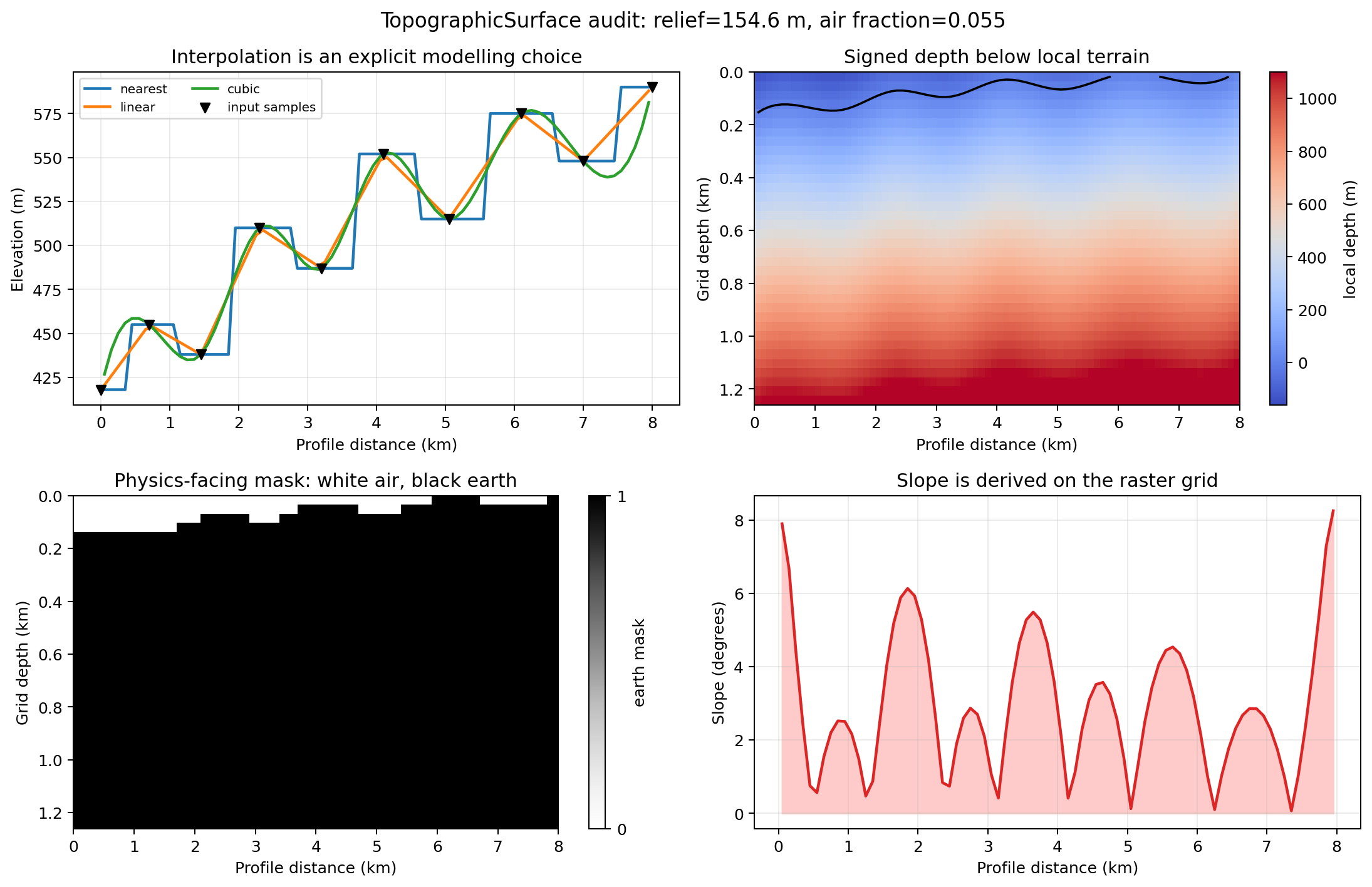
Executed terrain workflow from sparse elevation samples to the arrays used by a forward mesh.

Nearest interpolation preserves sample plateaus but produces discontinuous steps; linear interpolation is conservative between observations; cubic interpolation is smoother but can introduce extrema not present at a sample. Here the cubic raster spans 426.7–581.4 m even though the observations span 418–590 m because cell centres do not coincide with the endpoint samples. The signed-depth panel shows why surface_depth_m and local_depth_m must not be confused: the former is one terrain value per horizontal cell, while the latter broadcasts that surface across every depth cell. The binary mask is the geometry that a terrain-capable forward adapter would need; the slope curve is a diagnostic of the rasterization, not a replacement for inspecting the terrain itself. The distinction matters in the current stack: MT2DAdapter, MT3DAdapter, and the v1 ModEm3DAdapter all declare supports_topography=False and supports_inactive_cells=False. They reject an inactive air mask rather than silently solving terrain. Until a terrain-capable adapter is connected and benchmarked, these masks support geological auditing and display, not a claim of topographic Maxwell physics.

In the lower-right panel of the diagnostic, white cells lie above the black terrain line and are excluded by earth_mask(). The conductive and resistive lenses retain smooth transition shells, while the stratigraphic interfaces remain defined in the unwarped depth coordinate. The exact executable used for all four panels is included here; it also shows how the 32-realization variogram envelopes are assembled rather than hiding that ensemble step behind the finished image.

</>View geology-prior diagnostic source codeClick to inspect and copy the complete code

def make_geology_prior_diagnostic() -> None:
    """Visualise correlation recovery and compositional geological priors."""
    from pycsamt.ai.geology import (
        ElectricalLayer,
        EllipsoidalLens,
        GaussianCorrelation,
        GeologyGrid,
        directional_variogram,
        generate_gaussian_field,
        generate_layered_geology,
        insert_lenses,
        interpolate_topography,
    )

    grid = GeologyGrid.regular_2d(nx=64, nz=32, dx_m=100, dz_m=50)
    correlation = GaussianCorrelation(length_x_m=700, length_z_m=150)
    example = generate_gaussian_field(grid, correlation, seed=12)

    variograms_x = []
    variograms_z = []
    for seed in range(32):
        realization = generate_gaussian_field(grid, correlation, seed=seed)
        variograms_x.append(
            directional_variogram(realization, "x", max_lag_cells=21).semivariance
        )
        variograms_z.append(
            directional_variogram(realization, "z", max_lag_cells=15).semivariance
        )
    variograms_x = np.asarray(variograms_x)
    variograms_z = np.asarray(variograms_z)
    lag_x = np.arange(1, 22) * 100.0
    lag_z = np.arange(1, 16) * 50.0

    layers = (
        ElectricalLayer(
            "weathered cover", 30.0, log10_std=0.10,
            heterogeneity=GaussianCorrelation(500, 120),
            resistivity_bounds_ohm_m=(8.0, 120.0),
        ),
        ElectricalLayer("sedimentary unit", 180.0),
        ElectricalLayer(
            "basement", 1200.0, log10_std=0.12,
            heterogeneity=GaussianCorrelation(900, 180),
            resistivity_bounds_ohm_m=(300.0, 4000.0),
        ),
    )
    layered = generate_layered_geology(
        grid,
        layers,
        [350.0, 950.0],
        seed=24,
        interface_relief_std_m=[60.0, 110.0],
        interface_correlation=GaussianCorrelation(850, 150),
        minimum_thickness_m=100.0,
    )
    lenses = (
        EllipsoidalLens(
            "conductor", 2100.0, 650.0, 650.0, 170.0, 6.0,
            dip_deg=12.0, transition_fraction=0.25,
        ),
        EllipsoidalLens(
            "resistor", 4700.0, 1150.0, 520.0, 210.0, 3500.0,
            dip_deg=-18.0, transition_fraction=0.20,
        ),
    )
    composed = insert_lenses(layered, lenses, conflict_policy="error")
    topo_x = np.linspace(0.0, 6400.0, 9)
    topo_elevation = 420.0 + 70.0 * np.sin(topo_x / 900.0) + 25.0 * np.cos(
        topo_x / 430.0
    )
    surface = interpolate_topography(
        grid, topo_x, topo_elevation, source="synthetic survey",
        interpolation_method="cubic",
    )

    fig, axes = plt.subplots(2, 2, figsize=(12.2, 8.4))
    extent = [0.0, 6.4, 1.6, 0.0]
    image = axes[0, 0].imshow(
        example.values, extent=extent, aspect="auto", cmap="RdBu_r",
        vmin=-2.5, vmax=2.5,
    )
    axes[0, 0].set(
        title="One standardized anisotropic Gaussian field",
        xlabel="Profile distance (km)", ylabel="Depth (km)",
    )
    fig.colorbar(image, ax=axes[0, 0], label="Standard deviations")

    ax = axes[0, 1]
    for lag, values, length, label, color in (
        (lag_x, variograms_x, 700.0, "x direction", "#2563eb"),
        (lag_z, variograms_z, 150.0, "z direction", "#dc2626"),
    ):
        normalized_lag = lag / length
        median = np.median(values, axis=0)
        lower, upper = np.percentile(values, [10, 90], axis=0)
        ax.plot(normalized_lag, median, "o-", color=color, label=f"{label}: median")
        ax.fill_between(normalized_lag, lower, upper, color=color, alpha=0.16)
    theory_lag = np.linspace(0.0, 3.1, 180)
    ax.plot(
        theory_lag, 1.0 - np.exp(-0.5 * theory_lag**2),
        "k--", lw=1.5, label="requested Gaussian model",
    )
    ax.set(
        title="32-realization directional variogram audit",
        xlabel="Lag / requested correlation length", ylabel="Semivariance",
        xlim=(0, 3.1), ylim=(0, 1.65),
    )
    ax.grid(alpha=0.25)
    ax.legend(fontsize=8)

    for ax, values, title in (
        (axes[1, 0], layered.resistivity_ohm_m, "Correlated interfaces + within-unit variability"),
        (axes[1, 1], composed.resistivity_ohm_m, "Lenses + interpolated topographic mask"),
    ):
        display = np.log10(values)
        if ax is axes[1, 1]:
            display = np.where(surface.earth_mask(), display, np.nan)
        image = ax.imshow(
            display, extent=extent, aspect="auto", cmap="viridis_r",
            vmin=0.6, vmax=3.7,
        )
        for interface in layered.interface_depth_m:
            ax.plot(grid.x_m / 1000.0, interface / 1000.0,
                    color="white", lw=0.9, alpha=0.75)
        if ax is axes[1, 1]:
            ax.plot(
                grid.x_m / 1000.0, surface.surface_depth_m / 1000.0,
                color="#111827", lw=1.4, label="terrain",
            )
            ax.legend(fontsize=8, loc="lower left")
        ax.set(title=title, xlabel="Profile distance (km)", ylabel="Depth (km)")
        fig.colorbar(image, ax=ax, label=r"$\log_{10}\rho$ [$\Omega\cdot$m]")

    fig.suptitle(
        "A geological prior is audited statistically, then composed geometrically",
        fontsize=13,
    )
    fig.tight_layout()
    _save(fig, "geology_prior_diagnostic.png")

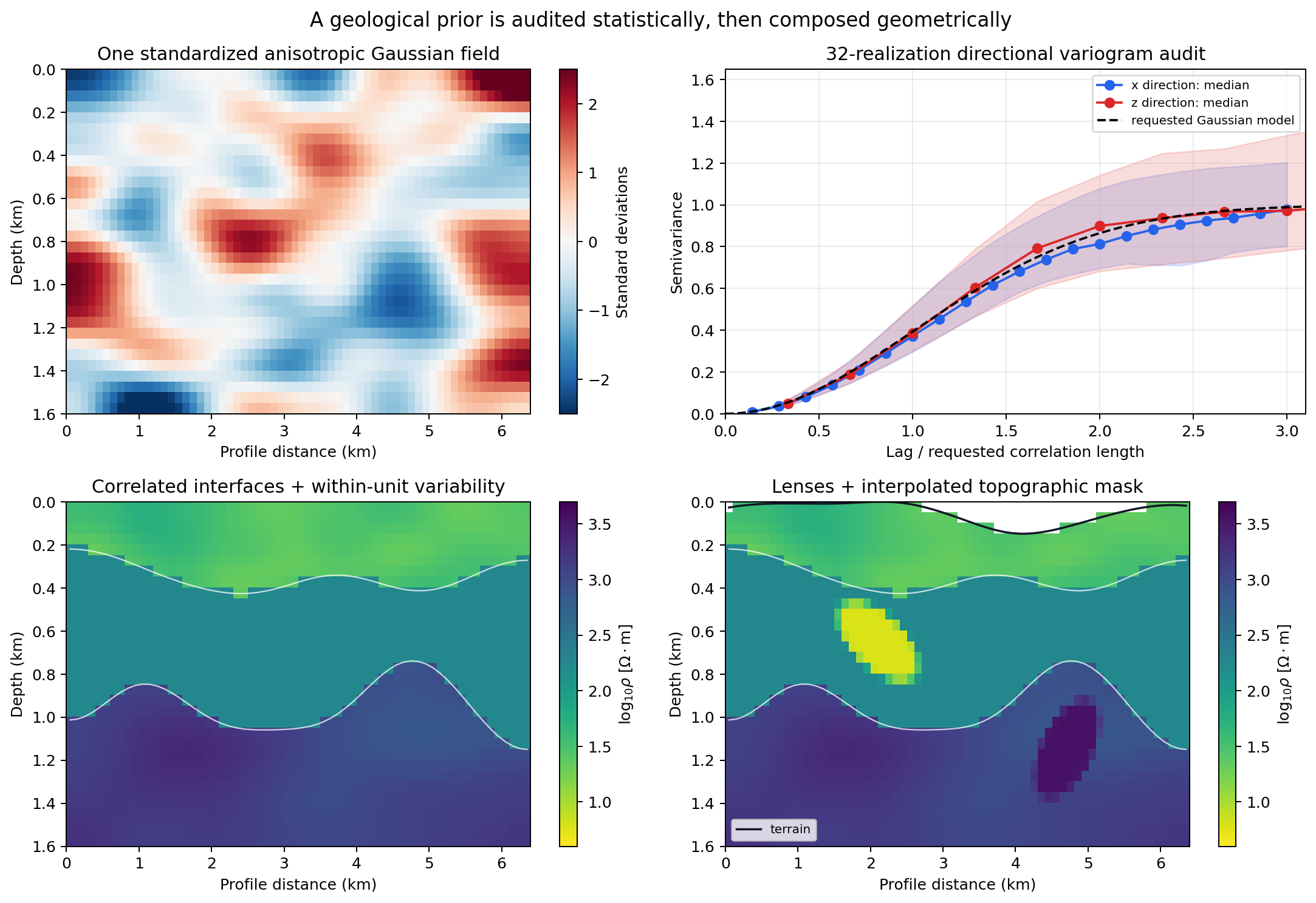
Statistical verification and geometric composition of a deterministic 2-D prior. Shaded variogram bands are the 10th–90th percentiles across 32 realizations, not uncertainty for one realization.

6.3.4.6. Carry the same composition into 3-D

A 3-D grid has canonical array shape (nz, ny, nx). Its GaussianCorrelation must supply length_y_m; azimuth_deg rotates the horizontal correlation axes. Likewise, a 3-D EllipsoidalLens supplies center_y_m and radius_y_m. Its azimuth rotates the horizontal major axis, while dip_deg rotates that major axis toward depth. These angles describe the prior geometry; they are not strike and dip estimates recovered from data.

This executable example builds correlated stratigraphy, inserts one dipping conductor, rasterizes a simple terrain plane from projected control points, and plots two vertical sections plus one horizontal slice. The named masks avoid relying on integer labels whose meaning may be forgotten later.

>>> import matplotlib.pyplot as plt
>>> import numpy as np
>>> from pycsamt.ai.geology import (
...     ElectricalLayer, EllipsoidalLens, GaussianCorrelation, GeologyGrid,
...     generate_layered_geology, insert_lenses, interpolate_topography,
... )
>>> grid3 = GeologyGrid.regular_3d(
...     nx=42, ny=30, nz=24, dx_m=150, dy_m=150, dz_m=60
... )
>>> correlation3 = GaussianCorrelation(
...     length_x_m=900, length_y_m=600, length_z_m=240, azimuth_deg=30
... )
>>> units3 = (
...     ElectricalLayer(
...         "cover", 35, log10_std=0.08, heterogeneity=correlation3
...     ),
...     ElectricalLayer("host", 420),
...     ElectricalLayer(
...         "basement", 1800, log10_std=0.10, heterogeneity=correlation3
...     ),
... )
>>> layered3 = generate_layered_geology(
...     grid3, units3, [360, 900], seed=31,
...     interface_relief_std_m=[70, 120],
...     interface_correlation=correlation3,
...     minimum_thickness_m=120,
... )
>>> body3 = EllipsoidalLens(
...     "dipping conductor", center_x_m=3300, center_y_m=2250,
...     center_z_m=690, radius_x_m=1150, radius_y_m=650,
...     radius_z_m=260, resistivity_ohm_m=8, azimuth_deg=35,
...     dip_deg=18, transition_fraction=0.22,
... )
>>> volume3 = insert_lenses(layered3, [body3], conflict_policy="error")
>>> grid3.shape, layered3.interface_depth_m.shape
((24, 30, 42), (2, 30, 42))
>>> int(volume3.lens_mask("dipping conductor").sum())
604
>>> round(volume3.summary()["assigned_fractions"]["dipping conductor"], 4)
0.02
>>> layered3.layer_mask("host").shape, layered3.interface(0).shape
((24, 30, 42), (30, 42))
>>>
>>> xy = np.array([
...     [0, 0], [6300, 0], [0, 4500], [6300, 4500],
...     [3150, 2250], [1575, 1125], [4725, 3375],
... ])
>>> elevation = 510 + 0.018 * xy[:, 0] - 0.012 * xy[:, 1]
>>> terrain3 = interpolate_topography(
...     grid3, xy, elevation, source="projected control points"
... )
>>> log_rho = np.log10(volume3.resistivity_ohm_m)
>>> earth = terrain3.earth_mask()
>>> iy, ix = grid3.shape[1] // 2, grid3.shape[2] // 2
>>> iz = int(np.argmin(np.abs(grid3.z_m - body3.center_z_m)))
>>> views = (
...     np.where(earth[:, iy, :], log_rho[:, iy, :], np.nan),
...     np.where(earth[:, :, ix], log_rho[:, :, ix], np.nan),
...     log_rho[iz],
... )
>>> fig, axes = plt.subplots(1, 3, figsize=(13.8, 4.8))
>>> extents = ([0, 6.3, 1.44, 0], [0, 4.5, 1.44, 0], [0, 6.3, 4.5, 0])
>>> for ax, values, extent in zip(axes, views, extents):
...     image = ax.imshow(
...         values, extent=extent, aspect="auto", cmap="viridis_r",
...         vmin=0.7, vmax=3.4,
...     )
>>> colorbar_axis = fig.add_axes([0.925, 0.19, 0.015, 0.60])
>>> _ = fig.colorbar(
...     image, cax=colorbar_axis, label="log10 resistivity [ohm m]"
... )
>>> fig.subplots_adjust(
...     left=0.06, right=0.90, bottom=0.13, top=0.82, wspace=0.32
... )
>>> plt.show()

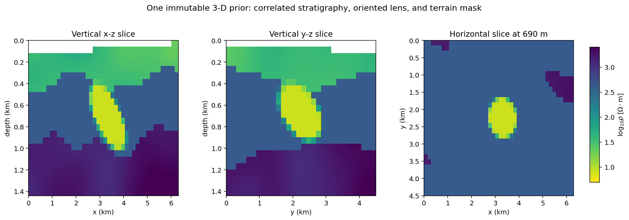
Executed 3-D composition shown with one shared resistivity scale.

The conductor appears with different widths and apparent inclinations in the two vertical sections because each plane cuts the same rotated ellipsoid at a different orientation. The horizontal slice exposes its azimuth more directly. White cells in the vertical views are air from terrain3.earth_mask(); they are not missing geological samples. Notice also that the body occupies only about 2% of the volume. That fraction should be checked across an ensemble: a rare target can be scientifically plausible yet too uncommon for a network to learn reliably.

6.3.4.7. Connecting a rich prior to 3-D Maxwell training

The composition above is available to a custom forward workflow, but it is not yet the distribution sampled by pycsamt.ai.training.dataset3d.generate_3d_maxwell_dataset(). That convenience generator currently draws one standardized Gaussian field and maps it affinely into log10(resistivity). Increasing n_realizations changes its random draws and correlation lengths; it does not introduce the named layers, projected interfaces, lens masks, or overlap policies demonstrated here. The 2-D Maxwell dataset generator has the same Gaussian-field boundary.

For a layered/lens corpus, generate and persist each LensGeology or LayeredGeology realization first, convert resistivity_ohm_m to conductivity, and explicitly transfer it from the geological grid to a padded solver mesh. Solve the resulting MaxwellProblem with the selected adapter, then retain the original geological volume as the target or resample it onto the declared output grid. In symbols,

(8)\[\boldsymbol{\sigma}_s =P_{g\rightarrow s}\!\left(\boldsymbol{\rho}_g^{-1}\right), \qquad \mathbf y_o=P_{g\rightarrow o}\!\left(\log_{10}\boldsymbol{\rho}_g\right).\]

The transfer operators, grid edges, model hash, station coordinates, forward problem hash, backend identity, and accepted or rejected solve status belong in the realization record. Nearest-cell extension into padding may be a reasonable explicit boundary convention; allowing array shapes to imply a mapping is not. Keep every corruption variant attached to the same parent model hash so variants cannot leak across dataset partitions.

Equation (8) also separates terrain display from terrain physics. Applying earth_mask only to a plotted target does not modify \(\boldsymbol{\sigma}_s\); a genuine terrain solve requires the mask to enter a backend that supports inactive cells and has been validated for that geometry.

6.3.4.8. Persist identity and audit the ensemble

Generated fields, layered models, lens models, and topographic surfaces are immutable and provide platform-stable hashes over their arrays and generation provenance. Their to_npz/from_npz methods use pickle-free archives and revalidate reconstructed geometry. A seed alone is insufficient: grid, boundary policy, correlation definition, layer parameters, overlap policy, and values all contribute to identity.

>>> from pathlib import Path
>>> from tempfile import TemporaryDirectory
>>> from pycsamt.ai.geology import (
...     CorrelatedField, LayeredGeology, LensGeology, TopographicSurface,
... )

>>> with TemporaryDirectory() as directory:
...     root = Path(directory)
...     field_copy = CorrelatedField.from_npz(
...         field.to_npz(root / "field.npz")
...     )
...     layer_copy = LayeredGeology.from_npz(
...         layered.to_npz(root / "layers.npz")
...     )
...     lens_copy = LensGeology.from_npz(
...         composed.to_npz(root / "lenses.npz")
...     )
...     surface_copy = TopographicSurface.from_npz(
...         surface.to_npz(root / "terrain.npz")
...     )
...     print(field_copy.field_hash == field.field_hash)
...     print(layer_copy.model_hash == layered.model_hash)
...     print(lens_copy.model_hash == composed.model_hash)
...     print(surface_copy.surface_hash == surface.surface_hash)
True
True
True
True

Before sending an ensemble to Solver-neutral Maxwell contracts, audit more than image quality: requested versus empirical variograms, resistivity histograms and bounds, layer and lens occupancy by depth, interface-adjustment fraction, overlap frequency, topographic air fraction and slope, and coverage of rare structural combinations. Split related corruptions or variants by shared realization lineage as explained in Canonical data contracts; otherwise nearly identical geology can leak across training and evaluation. These diagnostics test whether the sampler represents the intended prior. They do not prove that the intended prior represents the field area–that requires geological constraints and the domain-gap checks in Domain-gap and noise simulation.