4. Airborne Natural-Source EM: AFMAG, ZTEM, And MobileMT

CSAMT, AMT, and MT Overview and Field Zones: Near, Transition, And Far Field already make the key distinction that motivates this page: MT and AMT have no controlled transmitter to be close to or far from, so the near/transition/far dichotomy that governs CSAMT does not apply to them – their natural source is treated as a plane-wave field at essentially all usual survey scales. Every method on this page inherits that same property, then adds a second one: the receiver is airborne. A helicopter or fixed-wing aircraft tows one or more magnetic-field sensors along a flight line while a fixed ground station (or, for the historical instrument, nothing at all) provides the reference. No transmitter is switched on anywhere in the survey. This page explains why that combination works, what physical object each of the three systems pyCSAMT supports actually measures, and how those objects relate to the impedance-tensor formalism the rest of the documentation builds around. The worked, code-driven demonstrations live on their own pages – AFMAG Tilt-Angle Diagnostics And Motion-Coupling Physics and ZTEM Total-Divergence, Phase-Rotation, And Map-View Diagnostics. For a broader, general-audience introduction to how airborne and ground geophysical surveys are designed and read – useful background before the pyCSAMT-specific physics below – see UBC-GIF’s open Geophysical Surveys overview on GeoSci.xyz.

4.1. Why A Natural Source Can Be Flown

A grounded CSAMT transmitter radiates a field whose geometry depends on the transmitter-receiver offset, which is exactly why Field Zones: Near, Transition, And Far Field needs a near/transition/far classification at all. The natural audio-frequency field that AFMAG-family methods use has no such geometry to worry about: worldwide thunderstorm activity (the Schumann resonance source band) illuminates the whole survey area with what is, to a very good approximation, a uniform, planar, vertically incident wave [Ward1959] [Legault2012]. That is precisely the plane-wave assumption Impedance Tensor builds the tensor formalism on, and it is why an AFMAG-family instrument does not need a matched transmitter/receiver pair the way CSAMT does – only a receiver.

The same field diffuses downward and is attenuated on the skin-depth scale already derived in Maxwell Forward Modelling and Solver Contracts,

\[\delta \approx 503\sqrt{\rho/f}\ \mathrm{m}\]

((8)), which Legault et al. (2012, citing Vozoff 1972) quote in exactly this form when motivating ZTEM’s depth of investigation. A lower audio frequency therefore probes deeper, at the cost of a weaker natural signal and a coarser lateral footprint – the same trade-off that governs sounding-curve design in ground MT/AMT, now applied to the choice of which of a handful of fixed audio frequencies (typically a few tens to a few hundred Hz) an airborne survey flies.

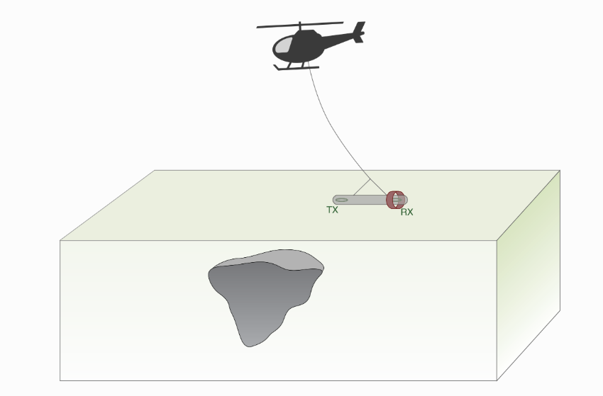
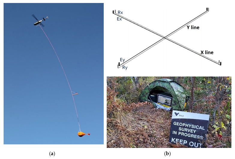
Conceptual layout of a helicopter-towed natural-source airborne EM survey: an airborne receiver bird flies a grid of flight lines while natural audio-frequency energy illuminates the whole survey area from above. AFMAG, ZTEM, and MobileMT differ in how many field components the bird carries, whether a temporary ground base station is required, and whether that ground station measures a magnetic or an electric field – the distinctions this page works through below.

Because there is no controlled source, an airborne AFMAG-family survey also inherits the caution Field Zones: Near, Transition, And Far Field raises for ground MT/AMT rather than its own: the relevant risk is not a near-field bias but static-shift-like galvanic distortion and, uniquely to the airborne case, motion-induced noise from the bird’s own attitude (covered below).

4.2. From A Scalar Tilt Angle To A Tensor

Ward (1959) introduced AFMAG as a two-coil comparator: one coil tuned to the local vertical, one to the horizontal, with the operator reading a single tilt/deflection angle at each station. That angle carries real information – it responds to the same subsurface conductivity contrasts a modern tensor system does – but it is a scalar, with no polarization-ellipse decomposition and no way to separate the response into orthogonal components. pycsamt.airborne.afmag keeps this historical reading as its own first-class shape rather than forcing it into a tensor container it cannot honestly fill; see AFMAG Tilt-Angle Diagnostics And Motion-Coupling Physics for a worked example built on a real digitised Ward (1959) field curve.

Pedersen et al. (1994) took the conceptually next step for the VLF band: a tensor instrument relating a fixed ground-reference horizontal magnetic field to an airborne three-component field, giving a genuine Interstation transfer function rather than a bare angle,

(1)\[\begin{split}\begin{pmatrix} H_x \\ H_y \\ H_z \end{pmatrix}_{r} = \begin{pmatrix} H_{xx} & H_{xy} \\ H_{yx} & H_{yy} \\ H_{zx} & H_{zy} \end{pmatrix} \begin{pmatrix} H_x \\ H_y \end{pmatrix}_{r_0}\end{split}\]

(the same relation (1) states for modern tensor AFMAG/AirMt in AFMAG Tilt-Angle Diagnostics And Motion-Coupling Physics). ZTEM (Z-axis Tipper Electromagnetics; Lo and Zang 2008) specializes this idea to the audio-frequency band and to a single output row: the airborne bird carries only a vertical-axis coil, and the ground station only the two horizontal coils, so the matrix above collapses to its bottom row – the familiar tipper relation

\[H_z(f) = T_{zx}(f)\,H_x(f) + T_{zy}(f)\,H_y(f)\]

((1)). This is why pyCSAMT reuses tipper machinery for both ground \(H_z\) measurements and ZTEM: mathematically, once the horizontal ground reference is fixed, an airborne \(H_z\) reading is a tipper, no matter how it was acquired.

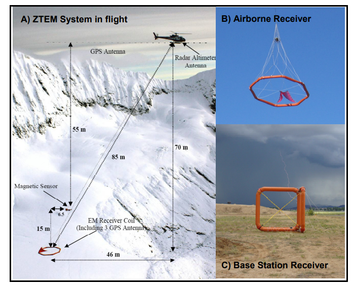
The ZTEM receiver bird in flight over the Gold Springs, Nevada survey, with the ground base-station coils shown alongside. The vertical-axis \(H_z\) receiver coil and its GPS antenna are towed roughly 55-85 m below and behind the helicopter; the fixed ground station (bottom right) records the horizontal reference field \(H_x, H_y\) throughout the flight. Reproduced from [Legault2012] , Fig. 4a.

Legault et al. (2012) flew exactly this configuration over the Gold Springs low-sulphidation epithermal gold-silver district in south-eastern Nevada – 41 east-west lines at 200 m spacing plus 6 tie lines, 470 line-km, at six frequencies from 30 to 720 Hz – and found that resistivity highs recovered from the tipper data, converted to a pseudo-section image, clustered around every known gold occurrence. That real survey (in the smaller, seven-line synthetic form committed as gold_springs_nv) is the worked example ZTEM Total-Divergence, Phase-Rotation, And Map-View Diagnostics builds on. Sattel and Witherly (2012) describe the complementary map-view processing – total divergence, phase rotation, and multi-line gridding – also demonstrated there; this theory page only summarizes the physics: the total-divergence / Peaker transform converts a raw tipper crossover, which is awkward to pick automatically from a map, into a peak centred on the causative contact,

\[\mathrm{DT} = \frac{\partial T_{zx}}{\partial x},\]

a relation Lo and Zang (2008) derive and that Sattel and Witherly (2012) note coincides, for a single flight line, with Pedersen’s own VLF-era Peaker parameter. See Total divergence and ZTEM Total-Divergence, Phase-Rotation, And Map-View Diagnostics for the full derivation, worked numbers, and the map-view figures.

4.3. Why Attitude, Not Just Geology, Shows Up In The Data

A ground AFMAG or MT station is bolted to the earth; an airborne receiver bird is not. As the helicopter and bird yaw, pitch, and roll along the flight line, the sensor’s own coordinate frame rotates with respect to the (much larger) steady geomagnetic field, and that rotation projects a spurious signal into the measured components – signal that looks, to a naive processor, exactly like a subsurface response. Liu et al. (2018) formalize this with a sequence of rotation matrices carrying the field from the local geographic frame into the sensor’s own frame as a function of the platform’s instantaneous yaw, pitch, and roll angles.

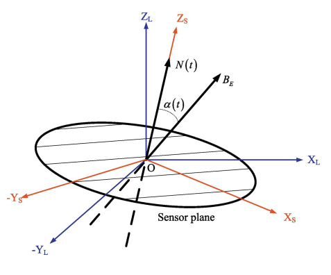
Geometry of motion-induced coupling: the sensor plane’s tilt angle \(\alpha(t)\) with respect to the local horizontal, driven by the airborne platform’s attitude, projects a component of the (otherwise DC) geomagnetic field into the measured signal. Reproduced from [Liu2018] , Fig. 1.

The key practical finding is that this motion-coupled noise concentrates at low frequency and grows with attitude amplitude and with the angle between the flight direction and the local geomagnetic field – exactly the frequency band where AFMAG-family methods also carry their deepest, most valuable signal, since low frequency means large skin depth in (8). There is consequently a genuine trade-off, not just an engineering inconvenience: gyro-stabilized bird mounts and post-flight attitude compensation can suppress the noise, but never perfectly, so the lowest usable frequency on a real survey is set as much by platform stability as by target depth. pycsamt.emtools.afmag implements Liu et al.’s rotation-matrix physics directly (motion_susceptibility_table(), flag_motion_susceptible_band()) so that a survey’s most exposed stations and frequency bands can be flagged before interpretation rather than after; AFMAG Tilt-Angle Diagnostics And Motion-Coupling Physics and ZTEM Total-Divergence, Phase-Rotation, And Map-View Diagnostics both show this in practice; the latter also masks frequencies outside the vendor-declared usable band directly (mask_outside_ztem_band()).

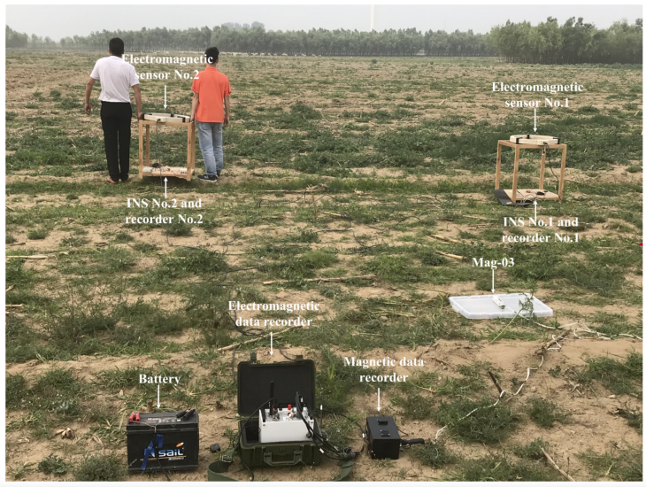
A real airborne AFMAG sensor package staged for a field test, with the EM sensor head, inertial navigation system (INS), and a Mag-03 fluxgate reference magnetometer visible – the same attitude and field-geometry instrumentation the motion-coupling model above is built from. Reproduced from [Liu2018] , Fig. 6.

4.4. MobileMT: A Genuinely Different Physical Object

Every method above is, once the ground reference is fixed, a magnetic-field-to-magnetic-field transfer function – structurally a tipper or an interstation tensor, never an impedance. MobileMT (Prikhodko et al. 2022) breaks that pattern deliberately. Instead of a second magnetic station, MobileMT keeps a fixed ground electric dipole pair (\(E_x, E_y\)) as its reference and relates it to the airborne bird’s three magnetic coils, giving a complex admittance tensor,

(2)\[\begin{split}\begin{pmatrix} H_x \\ H_y \\ H_z \end{pmatrix} = \begin{pmatrix} Y_{xx} & Y_{xy} \\ Y_{yx} & Y_{yy} \\ Y_{hzx} & Y_{hzy} \end{pmatrix} \begin{pmatrix} E_x \\ E_y \end{pmatrix}.\end{split}\]

Compare this with (1): the matrix shape is identical (3 rows, 2 columns), but the input columns are now an electric field rather than a magnetic one. That single substitution is what makes \(Y\) the reciprocal of the classical MT impedance tensor \(Z\) (which gives \(E\) from \(H\), see (2) in Impedance Tensor) rather than another tipper-shaped object. It is also why pyCSAMT deliberately refuses to convert a MobileMT admittance transfer function into an EDI: an EDI file has nowhere honest to put a ground electric reference alongside an airborne magnetic response, so pycsamt.emtools.mobilemt carries it instead through the AirborneEMDataset hierarchy, never through Site.

MobileMT’s two-part acquisition geometry: an airborne bird carrying three orthogonal magnetic-field receiver coils, referenced to a fixed ground electric-dipole transmitter/receiver pair (\(E_x, E_y\)) rather than to a second magnetic station. Reproduced from [Prikhodko2022] , Fig. 2.

In the limit where the airborne and ground sensors are co-located – never exactly true in practice, but the limit both Zhdanov et al. (2024) and Sattel et al. (2019) state explicitly as the theoretical basis for MobileMT’s derived apparent-resistivity product – the admittance tensor reduces to the ordinary MT admittance, \(Y = Z^{-1}\). Applying that identity to pyCSAMT’s own Berdichevsky-determinant convention for \(Z\) (pycsamt.z.resphase.ResPhase’s res_det/phase_det, the same \(\rho_a \approx 0.2\,|Z|^2/f\) shortcut already labelled (7), generalized from a single component to the full 2x2 determinant) and substituting \(\det Y = 1/\det Z\) gives, by direct algebra, a theoretical apparent conductivity and phase for the admittance tensor:

(3)\[\sigma_a = 5\,f\,|\det Y|, \qquad \varphi_a = -\arg\sqrt{\det Y}.\]

The leading constant, \(5 = 1/0.2\), is the same empirical Zonge-style factor as (7), simply inverted because the tracked quantity is now a conductivity rather than a resistivity. admittance_determinant_table() implements (3) directly. It is worth being explicit about what this quantity is not: it is a theoretical, co-located-sensor-limit conductivity derived from pyCSAMT’s own determinant convention, not a reproduction of MobileMT’s proprietary processed apparent-conductivity product. When a delivered dataset already carries that vendor-processed quantity, pycsamt.emtools.mobilemt reports it alongside, unmodified, as apparent_conductivity_native_Sm, precisely so the two are never silently conflated.

A second, scale-invariant diagnostic needs no physical constant at all and is therefore safe to compute directly from any admittance tensor, including a non-co-located one: a Swift (1967)-style skew ratio applied to the horizontal 2x2 admittance sub-block by direct algebraic analogy with the impedance-tensor skew already used elsewhere in pyCSAMT (see Dimensionality, Distortion, And The Phase Tensor),

(4)\[\mathrm{skew}_Y = \frac{|Y_{xx}+Y_{yy}|}{|Y_{xy}-Y_{yx}|}.\]

A low value indicates a tensor close to the ideal 1-D/2-D-consistent form; a large value signals departure from that form – instrument coupling error, genuine 3-D structure, or non-co-located-sensor geometry effects that (3)’s co-located assumption does not capture. admittance_skew_table() implements (4).

Zhdanov et al. (2024) demonstrate the practical payoff of this formalism on a real 3-D case: jointly inverting MobileMT admittance data with total-magnetic-intensity (TMI) magnetic data over a Climax-style porphyry molybdenum-copper breccia pipe target in East Greenland, recovering a coincident resistivity-low/susceptibility-high body consistent with the known alteration geometry. The synthetic flammefjeld_greenland sample dataset committed under data/mobileMT/ is loosely inspired by that survey; the KL-22 kimberlite pipe survey of Prikhodko et al. (2022) and Sattel et al. (2019) motivates the companion timiskaming_kimberlite_on dataset.

4.5. Comparing The Three Systems

System	Source	Airborne channels	Ground reference	Response object
Classical AFMAG (Ward 1959)	Natural audio-frequency	1 (tilt/deflection angle)	None	Scalar angle – no tensor
Tensor AFMAG / AirMt	Natural audio-frequency	\(H_x, H_y, H_z\)	Fixed \(H_x, H_y\) station	Interstation transfer function, (1)
ZTEM	Natural audio-frequency	\(H_z\) only	Fixed \(H_x, H_y\) station	Tipper \((T_{zx}, T_{zy})\), (1)
MobileMT	Natural audio-frequency	\(H_x, H_y, H_z\)	Fixed \(E_x, E_y\) dipole pair	Admittance \(Y\), (2)

Every row shares the same natural, plane-wave-illuminated source and the same absence of a controlled transmitter; the columns that differ are exactly what changes which pyCSAMT container carries the data (Site and pycsamt.emtools.ztem/ pycsamt.emtools.afmag for the magnetic-only rows, versus AirborneEMDataset and pycsamt.emtools.mobilemt for the admittance row) and which derived quantities are physically meaningful for it. A tipper or interstation tensor has no natural resistivity/phase product because it never involves an electric field; only the admittance tensor does, through (3).

4.6. Practical Implications

A few consequences follow directly from the physics above and are worth stating explicitly before using any of the three systems’ along-line diagnostics:

Warning

The total-divergence, phase-rotation, and crossover diagnostics summarized above (and implemented in pycsamt.emtools.ztem) all project stations onto a single along-line bearing. Passing a multi-line survey to any of them without first grouping by flight line silently differentiates or compares across line boundaries rather than along one coherent profile. select() and the LineId survey metadata exist precisely to make that grouping explicit; see ZTEM Total-Divergence, Phase-Rotation, And Map-View Diagnostics for the pattern.

Note

Neither classical tilt-angle AFMAG nor a bare tipper/interstation tensor has a closed-form apparent-resistivity relation – unlike full MT, there is no electric-field channel to form a ratio against. Only MobileMT’s admittance tensor supports (3), and even then only as a theoretical, co-located-sensor-limit quantity, not a substitute for a vendor-delivered product.

Important

Motion-induced noise and the finite usable frequency band are not optional caveats: they set the practical lower bound on investigation depth for every system on this page, often more tightly than the target’s own conductivity does. Always mask or flag frequencies outside a system’s declared usable band (mask_outside_ztem_band(), mask_outside_mobilemt_band()) before interpreting a total-divergence map or a resistivity pseudo-section.

4.7. Next Steps

For worked, code-driven demonstrations built on real synthetic surveys, continue with:

• AFMAG Tilt-Angle Diagnostics And Motion-Coupling Physics – both AFMAG response families, motion-noise diagnostics, and the amplification parameter, on a digitised Ward (1959) curve and a modern tensor AirMt survey.

• ZTEM Total-Divergence, Phase-Rotation, And Map-View Diagnostics – total divergence, phase rotation, and multi-line map gridding, on the Gold Springs and Forrestania surveys.

• pycsamt.emtools.mobilemt – admittance, determinant apparent conductivity, and skew diagnostics on the Flammefjeld and Timiskaming synthetic surveys.

4.8. References

The physics and figures above draw directly on [Ward1959], [Liu2018], [Lo2008], [Legault2012], [Sattel2012], [Pedersen1994], [Prikhodko2022], [Sattel2019], [Zhdanov2024], and [Swift1967]. See References for full citations.