
11.15. ZTEM Total-Divergence, Phase-Rotation, And Map-View Diagnostics#
ZTEM (Z-axis Tipper Electromagnetic; Lo and Zang 2008) is an airborne variant of AFMAG: a helicopter-towed vertical-field (\(H_z\)) coil is referenced to fixed-ground horizontal-field (\(H_x\), \(H_y\)) base-station coils, giving the same tipper relationship AFMAG Tilt-Angle Diagnostics And Motion-Coupling Physics already introduces,
Two real surveys motivate this page: Legault et al. (2012) flew a
ZTEM/magnetics survey over the Gold Springs low-sulphidation
epithermal gold-silver district in south-eastern Nevada, and Sattel
and Witherly (2012) processed a ZTEM data set from the Forrestania,
Western Australia EM test range (two drilled massive-sulphide bodies,
IR2 and IR4). pycsamt.emtools.ztem implements the specific
along-profile and map-view processing both papers describe: total
divergence (the Peaker), Hilbert-transform phase rotation, and
multi-line map gridding. This page covers all three, on top of the
data model Airborne EM Guide introduces
(pycsamt.airborne.ztem and
AirborneSite carry ZTEM data honestly
– no electric channel, no EDI bridge, no impedance requirement),
using the two committed synthetic sample surveys that demonstrate
them, gold_springs_nv (a real 7-line, 105-station block survey)
and forrestania_wa (a single 15-station line).
11.15.1. Building A ZTEM Response#
build_ztem_line() accepts a
NavigationTrack and a line-batched complex
tipper array and returns one flight line with one
EMTF document per sample – the same
construction pattern AFMAG Tilt-Angle Diagnostics And Motion-Coupling Physics uses. The example below
builds a small nine-station line with a seeded synthetic crossover
anomaly:
>>> import numpy as np
>>> from pycsamt.airborne import NavigationTrack
>>> from pycsamt.airborne.ztem import build_ztem_line, ZTEMSystemSpec
>>> rng = np.random.default_rng(11)
>>> nav = NavigationTrack(
...     sample_ids=tuple(f"S{i:02d}" for i in range(9)),
...     easting=np.arange(9, dtype=float) * 50.0,
...     northing=np.zeros(9),
... )
>>> freqs = np.array([30.0, 45.0, 90.0, 180.0, 360.0, 720.0])
>>> x = np.arange(9, dtype=float) * 50.0
>>> x0 = float(np.median(x))
>>> shape = (x - x0) / 100.0 * np.exp(-(((x - x0) / 100.0) ** 2))
>>> tipper = np.zeros((9, 6, 2), dtype=complex)
>>> for k in range(6):
...     tipper[:, k, 0] = 0.15 * shape + 0.05j * shape
...     tipper[:, k, 1] = 0.03 * shape - 0.01j * shape
>>> tipper += 0.01 * (
...     rng.normal(size=tipper.shape) + 1j * rng.normal(size=tipper.shape)
... )
>>> line = build_ztem_line(
...     "DEMO01", nav, tipper, frequency=freqs,
...     system_spec=ZTEMSystemSpec(),
... )
>>> line.n_records
9
>>> record = line.get_record("S04")
>>> tf = record.emtf.get_transfer_function("tipper")
>>> np.round(tf.data[2], 4)  # 90 Hz, at the crossover centre
array([[0.0063+0.0039j, 0.004 +0.0046j]])
Station S04 sits exactly at the profile’s median position, the
crossover centre, so its tipper is dominated by noise rather than
signal – a useful sanity check that the synthetic construction
actually crosses zero where intended, confirmed properly with real
survey data next.
11.15.2. Reading The Sample Surveys#
ensure_asites() reads either committed
survey straight from its directory:
>>> from pycsamt.airborne.site import ensure_asites
>>> gold_springs = ensure_asites("data/ZTEM/gold_springs_nv")
>>> len(gold_springs), gold_springs.technologies
(105, ('ztem',))
>>> forrestania = ensure_asites("data/ZTEM/forrestania_wa")
>>> len(forrestania)
15
gold_springs_nv is a real block survey: 7 parallel east-west
lines, 150 m apart, 15 stations each, at the same six frequencies
Legault et al. (2012) list (30, 45, 90, 180, 360, 720 Hz). The
synthetic target’s amplitude follows a Gaussian centred on the
survey’s own line 4 and taper toward lines 1 and 7 at the block’s
edges – a body of finite strike length, not an infinite 2-D
structure – so every single-line figure below reads line 4, where the
target response is strongest:
>>> line4 = gold_springs.select(
...     predicate=lambda s: (
...         s.emtf.metadata.get("notes", {})
...         .get("ZTEM", {})
...         .get("LineId")
...         == "gold_springs_nv_L4"
...     )
... )
>>> len(line4)
15
The flight-line identifier is not part of any standard EMTF-XML field
– it is stashed in EMTF.metadata["notes"]["ZTEM"]["LineId"] by
this page’s own data generator specifically so a bare directory
re-read can recover per-station line membership; a real vendor
delivery would not carry this key, and ensure_asites() never
assumes it does.
11.15.3. Raw In-Phase/Quadrature Crossover#
Legault et al. (2012, Fig. 6)’s own synthetic forward-model figure
over this same mushroom-shaped target plots the raw in-line tipper’s
in-phase and quadrature parts together, in percent, along the flight
line, and reads a negative-to-positive crossover directly above the
target at every frequency.
ztem_crossover_diagnostics() finds that
crossover programmatically, and
plot_ztem_tipper_profile() draws exactly
the figure this describes:
>>> from pycsamt.emtools.ztem import (
...     plot_ztem_tipper_profile, ztem_crossover_diagnostics,
... )
>>> diag = ztem_crossover_diagnostics(line4, frequency_hz=90.0)
>>> round(diag["crossover_real_m"], 1), round(diag["crossover_imag_m"], 1)
(336.8, 356.2)
>>> round(diag["peak_to_peak_real"], 4), round(diag["peak_to_peak_imag"], 4)
(0.1039, 0.0591)
>>> ax = plot_ztem_tipper_profile(line4, frequency_hz=90.0)
>>> ax.figure.savefig("user-guide-emtools-ztem-01.png", dpi=200, bbox_inches="tight")
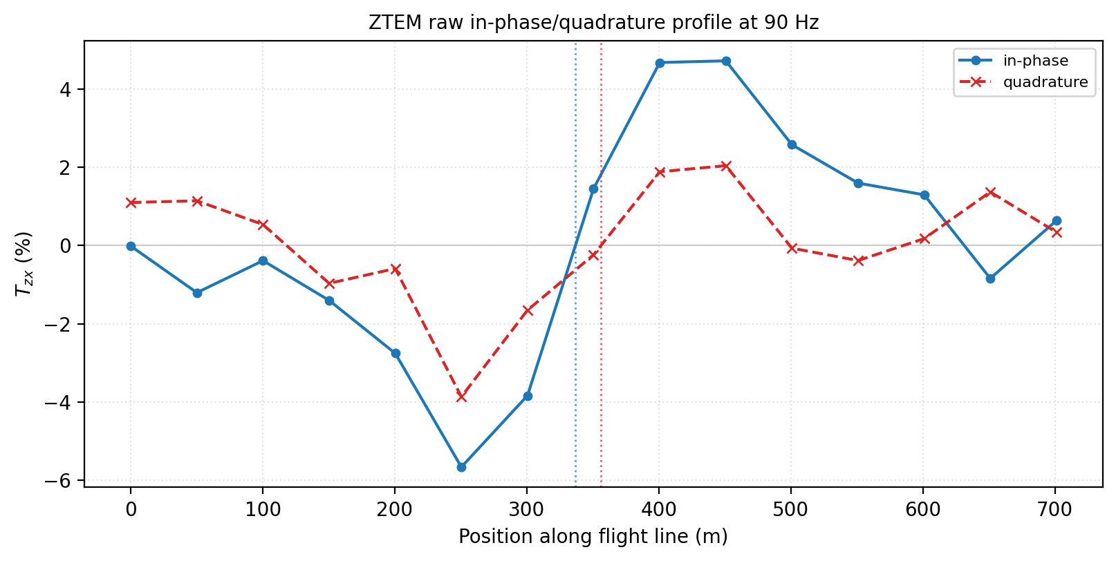
Raw in-phase/quadrature tipper profile, gold_springs_nv line 4
at 90 Hz, dotted lines marking each part’s crossover.#
Both parts cross zero within about 19 m of each other (337 m and
356 m along the line) – coherent, not the product of independent
noise – and both swing from a strong negative trough near station
GO_L4_005 to a strong positive peak near GO_L4_007, exactly
Legault et al. (2012)’s own description of the in-line response over
this target.
11.15.4. Total Divergence And Phase Rotation#
Sattel and Witherly (2012, Fig. 2) show that the same crossover
anomaly can be converted into a peak by two different, and for a
single flight line equivalent, spatial transforms: the along-line
horizontal derivative (Total Divergence, Lo and Zang 2008; the
VLF-style Peaker, Pedersen et al. 1994) and a Hilbert-transform phase
rotation. total_divergence_table() and
phase_rotate_table() implement each
directly:
>>> from pycsamt.emtools.ztem import total_divergence_table, phase_rotate_table
>>> dt = total_divergence_table(line4)
>>> dt.shape
(84, 9)
>>> list(dt.columns)
['station_a', 'station_b', 'x_m', 'dx_m', 'freq_hz', 'period_s', 'divergence_real', 'divergence_imag', 'divergence_abs']
>>> pr = phase_rotate_table(line4, frequency_hz=90.0)
>>> pr.shape
(64, 7)
>>> list(pr.columns)
['x_m', 'nearest_station', 'freq_hz', 'period_s', 'raw', 'rotated', 'envelope']
>>> from pycsamt.emtools.ztem import (
...     plot_ztem_divergence_profile, plot_ztem_phase_rotation_profile,
... )
>>> import matplotlib.pyplot as plt
>>> fig, (ax1, ax2) = plt.subplots(1, 2, figsize=(13.0, 4.2))
>>> _ = plot_ztem_divergence_profile(line4, frequency_hz=90.0, ax=ax1)
>>> _ = plot_ztem_phase_rotation_profile(line4, frequency_hz=90.0, ax=ax2)
>>> fig.tight_layout()
>>> fig.savefig("user-guide-emtools-ztem-02.png", dpi=200, bbox_inches="tight")
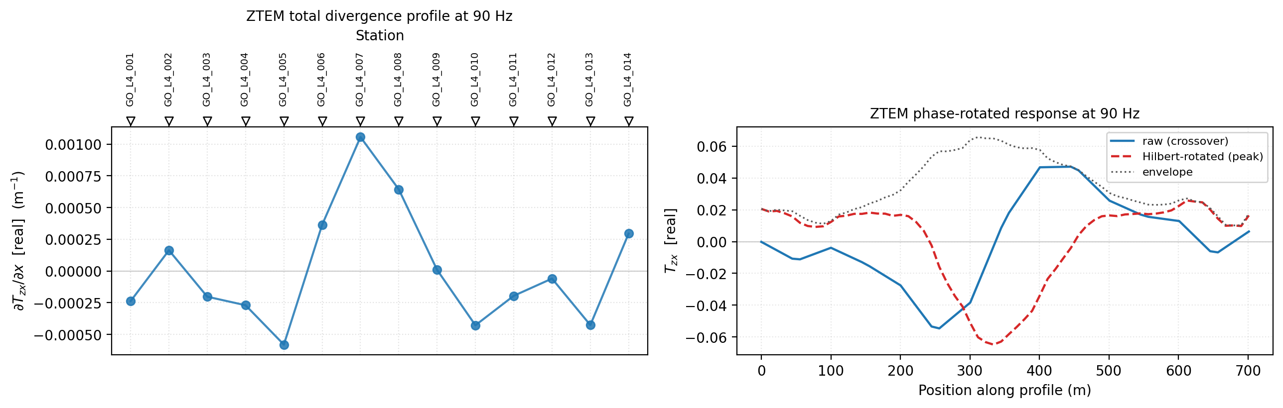
Left: total-divergence profile, gold_springs_nv line 4 at 90 Hz.
Right: the same station’s raw tipper (solid) alongside its
Hilbert-rotated peak and analytic-signal envelope (dashed/dotted).#
Both panels tell the same story two different ways. The divergence
profile peaks sharply at the station pair straddling the crossover
(GO_L4_006-GO_L4_007), the derivative’s largest magnitude
exactly where the raw curve changes sign fastest. The phase-rotation
panel shows the transformation directly: the raw curve (solid blue)
still crosses zero near 340-360 m, while its Hilbert-rotated
counterpart (dashed red) has already turned that crossing into a
trough, and the analytic-signal envelope (dotted grey) peaks squarely
over it – a single number per station that locates the anomaly
without requiring a reader to spot a sign change by eye.
11.15.5. Total Divergence Pseudosection#
A single-frequency profile hides how the crossover behaves with
period, and a single line hides how it varies across the survey.
plot_ztem_divergence_psection() images one
line’s every frequency at once, with the same cell-boundary-grid and
zero-level-contour overlay convention
plot_airmt_tilt_psection() introduced;
plot_ztem_divergence_psection_grid()
compares several lines side by side on one shared, zero-centred colour
scale (cmap="seismic", matplotlib’s scientific-notation tick
formatting so a colour range this small – values of order
\(10^{-4}\,\mathrm{m}^{-1}\) – reads as clean small integers with
a single x10^-4 multiplier rather than repeating 0.0001,
0.0002, … on every tick):
>>> from pycsamt.emtools.ztem import plot_ztem_divergence_psection_grid
>>> fig = plot_ztem_divergence_psection_grid(
...     gold_springs, max_lines=6, n_cols=3, cmap="seismic",
... )
>>> fig.savefig("user-guide-emtools-ztem-03.png", dpi=200, bbox_inches="tight")
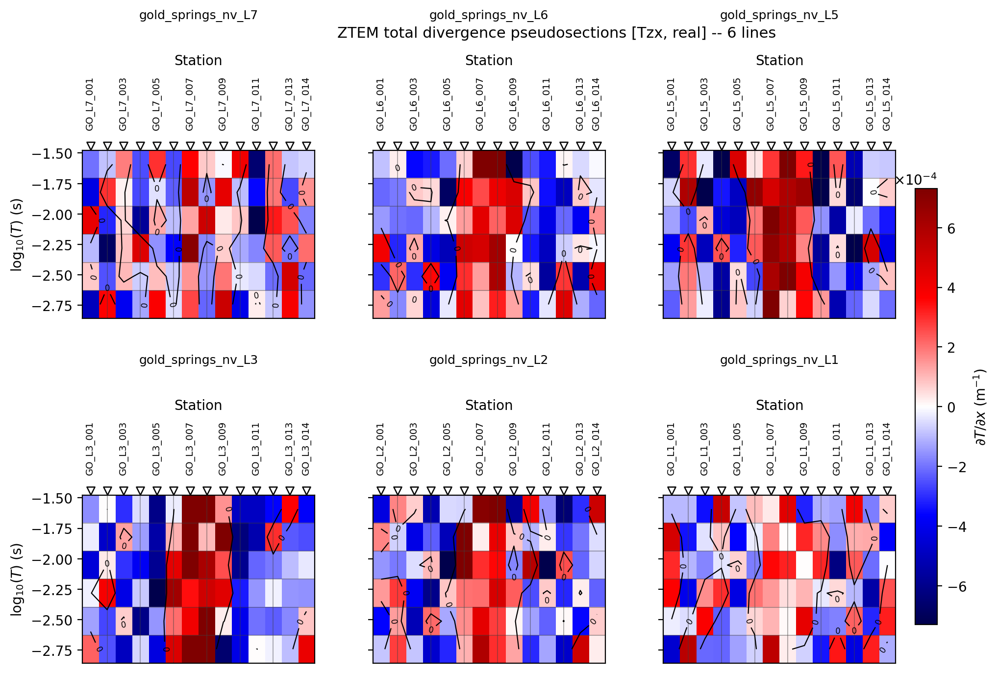
Total-divergence pseudosections for 6 of gold_springs_nv’s 7
lines (line 4 – already shown in detail above – is left out so
the remaining six can be compared against each other), one shared
colour scale, all six frequencies.#
Reading this alongside the per-line peak-to-peak amplitudes from Map-View Grids below tells a consistent story: lines 3, 5, and 6 – the closest neighbours of line 4’s target peak – each show a clear, coherent red column near stations 007-009 across every period, while lines 1, 2, and 7 – the survey’s outer edges – show weaker, noisier patterns with no single dominant column. The response is confined to a narrow station range rather than smearing or migrating with period on any of the six lines, the signature of a compact, shallow feature rather than a broad regional gradient.
11.15.6. Flight-Line Map#
Every function so far reads one flight line. gold_springs_nv’s 7
lines are a real plan-view survey, so
plot_ztem_flight_lines() – new alongside
this page, the Sattel and Witherly (2012, Fig. 7)-style navigation map
no other function in this project draws – shows them together:
>>> from pycsamt.emtools.ztem import plot_ztem_flight_lines
>>> ax = plot_ztem_flight_lines(gold_springs)
>>> ax.figure.savefig("user-guide-emtools-ztem-04.png", dpi=200, bbox_inches="tight")
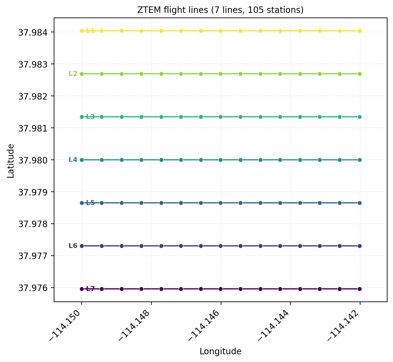
All 7 flight lines, gold_springs_nv, 150 m line spacing, each
coloured and labelled distinctly.#
Lines are recovered from station geometry alone (whichever of
longitude/latitude clusters into fewer, more widely separated groups
is treated as the cross-line axis), not from any stored line
identifier – a real, general heuristic for a parallel, axis-aligned
survey block like this one, not a claim of handling arbitrary flight
geometry. Each line’s label – L1 through L7 here – comes
from the real LineId metadata when present (with the survey’s own
common prefix stripped for legibility) rather than the detection
order, so these labels line up with “line 4” and the other line
numbers used throughout this page; a survey with no such metadata
falls back to a purely geometric L1, L2, … in detected-group
order instead.
11.15.7. Map-View Grids#
The genuine multi-line map product both papers show – Legault et al.
(2012, Fig. 7)’s “90 Hz In-Phase DT map”, Sattel and Witherly (2012,
Fig. 8-11)’s “XIP”/phase-rotated grids – interpolates one scalar field
across every line onto a regular map grid.
plot_ztem_map() does this for either the
raw tipper or the total-divergence field, differentiating each
detected line separately before pooling the result (a genuine
correctness requirement: differentiating across a line boundary would
produce a meaningless value, so this function – unlike
total_divergence_table() itself, which
assumes a single line – groups by line internally):
>>> from pycsamt.emtools.ztem import plot_ztem_map
>>> fig, (ax1, ax2) = plt.subplots(1, 2, figsize=(13.0, 6.0), sharey=True)
>>> _ = plot_ztem_map(gold_springs, quantity="tipper", frequency_hz=90.0, ax=ax1)
>>> _ = plot_ztem_map(gold_springs, quantity="divergence", frequency_hz=90.0, ax=ax2)
>>> _ = ax2.set_ylabel("")
>>> ax2.tick_params(axis="y", labelleft=False)
>>> fig.tight_layout()
>>> fig.savefig("user-guide-emtools-ztem-05.png", dpi=200, bbox_inches="tight")
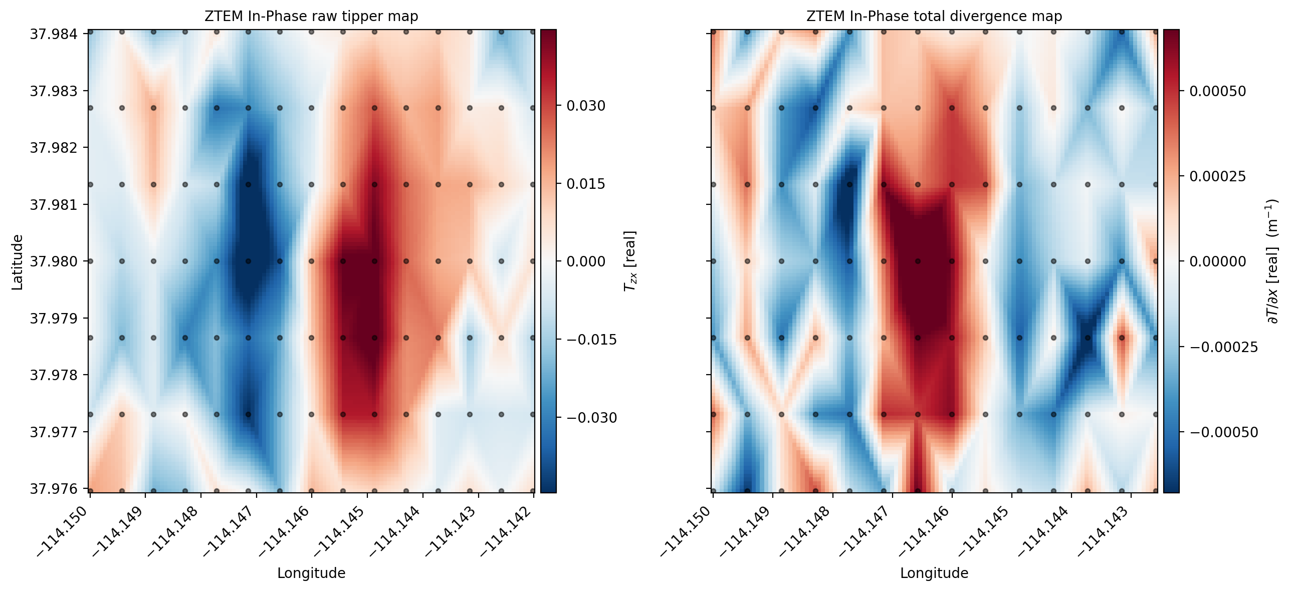
Left: raw in-phase tipper map. Right: total-divergence map. Both,
gold_springs_nv, 90 Hz, sharing one latitude axis (sharey)
since both panels cover the same stations.#
Both maps show the same north-south trending, roughly 150 m-wide resistive band, thickest around the survey’s middle latitudes and tapering toward both ends – Legault et al. (2012)’s own “cluster of resistive areas … suggesting separate epithermal cells” reading, reproduced here from a single, deliberately finite-strike-length target rather than several. The per-line peak-to-peak amplitude confirms the same pattern numerically, not just visually:
>>> for li in range(1, 8):
...     lid = f"gold_springs_nv_L{li}"
...     line = gold_springs.select(
...         predicate=lambda s, lid=lid: (
...             s.emtf.metadata.get("notes", {})
...             .get("ZTEM", {})
...             .get("LineId")
...             == lid
...         )
...     )
...     diag = ztem_crossover_diagnostics(line, frequency_hz=90.0)
...     print(f"L{li}: {diag['peak_to_peak_real']:.4f}")
L1: 0.0323
L2: 0.0603
L3: 0.0963
L4: 0.1039
L5: 0.0837
L6: 0.0812
L7: 0.0390
The amplitude rises smoothly from line 1 to a maximum at line 4 – where every single-line figure on this page reads its data – then falls back down by line 7, a clean Gaussian-shaped along-strike profile. This is the map view’s real payoff: no single-line figure above could show that lines 1 and 7 sit essentially off the target entirely, while lines 3-6 sit on top of it.
11.15.8. Masking The Usable Band#
mask_outside_ztem_band() reuses the
survey’s own published usable bandwidth
(ZTEMSystemSpec’s
practical_frequency_range_hz, 22-720 Hz by default) rather than
inventing a QC band – the same mask-only pipeline contract
flag_motion_susceptible_band() and
mask_outside_mobilemt_band() already
use. An explicit, narrower band shows the effect directly on
forrestania_wa:
>>> from pycsamt.emtools.ztem import mask_outside_ztem_band, plot_ztem_band_mask_psection
>>> masked = mask_outside_ztem_band(forrestania, band_hz=(40.0, 300.0))
>>> type(masked).__name__, len(masked)
('AirborneSites', 15)
>>> masked[0].freq
array([ 30.,  45.,  90., 180., 360., 720.])
>>> np.isfinite(masked[0].tipper[:, 0, 0].real)
array([False,  True,  True,  True, False, False])
>>> fig = plot_ztem_band_mask_psection(forrestania, band_hz=(40.0, 300.0))
>>> fig.savefig("user-guide-emtools-ztem-06.png", dpi=200, bbox_inches="tight")
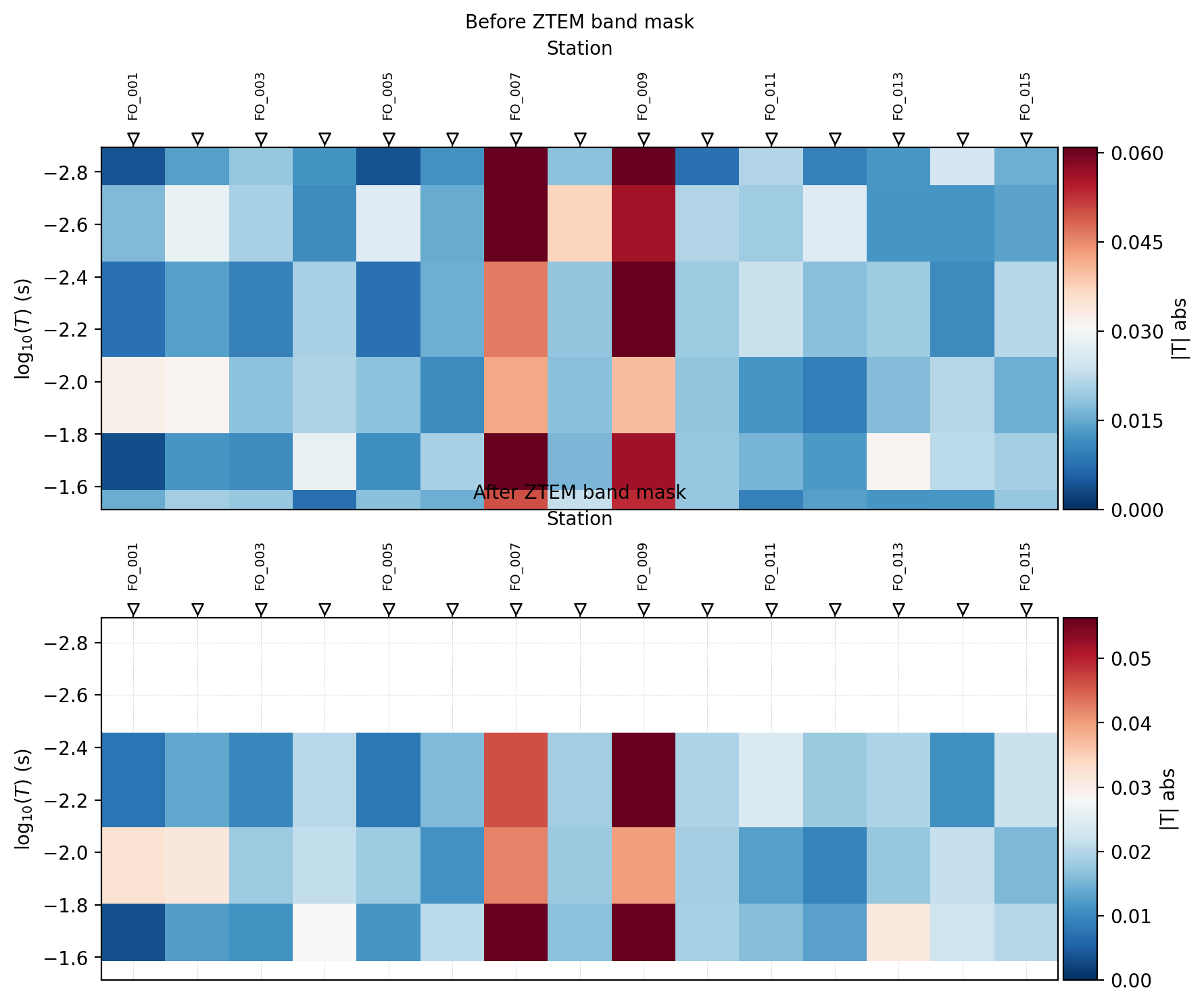
Before/after \(|T|\) pseudosection, forrestania_wa, masking
everything outside 40-300 Hz.#
The frequency axis and every station’s identity are unchanged by
masking – only the 30, 360, and 720 Hz rows turn blank (nan, not
a fabricated zero) in the lower panel, exactly the three frequencies
numpy.isfinite() marked False above.
Warning
Every file under data/ZTEM/ is synthetic, forward-modeled from
a simplified skin-depth-weighted analytic approximation – not
a vendor delivery sample and not a reproduction of either cited
paper’s actual field data. Each generated EMTF.description
states this explicitly. No proprietary ZTEM archive format is
parsed anywhere in pyCSAMT; pycsamt.airborne.ztem only maps
already-decoded arrays onto the common model.
11.15.9. Recommended Workflow#
The dropdown below reproduces every figure on this page end to end,
from the two ensure_asites calls through the map-view grids:
View the executed workflow source codeClick to inspect and copy the complete code
1def run_emtools_ztem_workflow() -> None:
2    gs_all, gs_l4, forrestania = _load_sites()
3    make_tipper_profile(gs_l4)
4    make_divergence_and_phase_rotation(gs_l4)
5    make_divergence_psection_grid(gs_all)
6    make_flight_lines(gs_all)
7    make_maps(gs_all)
8    make_band_mask(forrestania)
11.15.10. References#
ZTEM’s own general theory follows Lo and Zang (2008) [Lo2008], itself an airborne variant of [Ward1959]’s AFMAG. The Gold Springs synthetic target and its dual-frequency-style in-phase/ quadrature crossover reading follow [Legault2012]. The total divergence, phase rotation, and map-view diagnostics all follow [Sattel2012], who also credit the Peaker to [Pedersen1994] and the Total Divergence formulation to [Lo2008]. See [wang2025] for a recent 3-D staggered-grid ZTEM forward-modelling treatment, and AFMAG Tilt-Angle Diagnostics And Motion-Coupling Physics for the shared AFMAG tipper equivalence and the motion-coupling physics this page does not repeat.