Maps And Profiles#

The desktop map and profile viewers are the two fastest ways to check whether a loaded survey is spatially coherent and physically plausible. Use the map viewer to inspect station geometry, coordinate systems, elevation, apparent resistivity, and depth slices. Use the profile viewer to inspect station responses, pseudosections, tipper behaviour, phase tensors, and 2-D sections.

Both viewers use the active survey loaded in the main desktop session. They do not open a separate copy of the data; station selections and loaded Sites objects are shared with the station table and downstream workflow windows.

Recommended Inspection Order#

Use the viewers in a fixed order when opening a new line. It keeps visual interpretation from running ahead of basic data checks:

Station map – confirm that station positions and labels are sensible.
Elevation map – check whether elevation metadata are present and continuous along the line.
Single-station profile – inspect rho_a and phase curves for a few representative stations.
Pseudosections – look for line-scale continuity and frequency gaps.
Depth or resistivity maps – use interpolated maps only after station geometry and response curves look credible.
Phase tensor and tipper tabs – check dimensionality and directionality before strike analysis or 2-D inversion assumptions.

This order is intentionally conservative. A filled contour map can look convincing even when a coordinate system, station order, or component selection is wrong.

Open The Viewers#

After loading EDI data, open the viewers from the main toolbar:

Map opens the station and spatial-property map viewer.
Profile opens the per-station response and profile-section viewer.
Selecting a station in the main station table also updates the viewers when they are open.
Double-clicking or using Open Profile from the station detail card is a convenient way to jump directly to one station response.

The viewers remember their window geometry in the desktop session, so a saved session can restore a familiar inspection layout.

Viewer State And Active Survey#

The map and profile windows are listeners on the desktop session. When new data are loaded, the main window sends the loaded Sites object and station summary table to open panel windows. This means:

reloading data replaces the viewer content;
station selections are synchronized across the main table, map, profile viewer, and station detail card;
exported figures reflect the current viewer settings, not a separate saved analysis state;
saving the desktop session remembers layout and preferences, while the EDI files remain the source of scientific data.

Map Viewer Overview#

The map viewer starts with station geometry. This is the first map to inspect after loading a survey because it shows whether station order, line grouping, and coordinates make sense before any interpolation or geophysical colouring is applied.

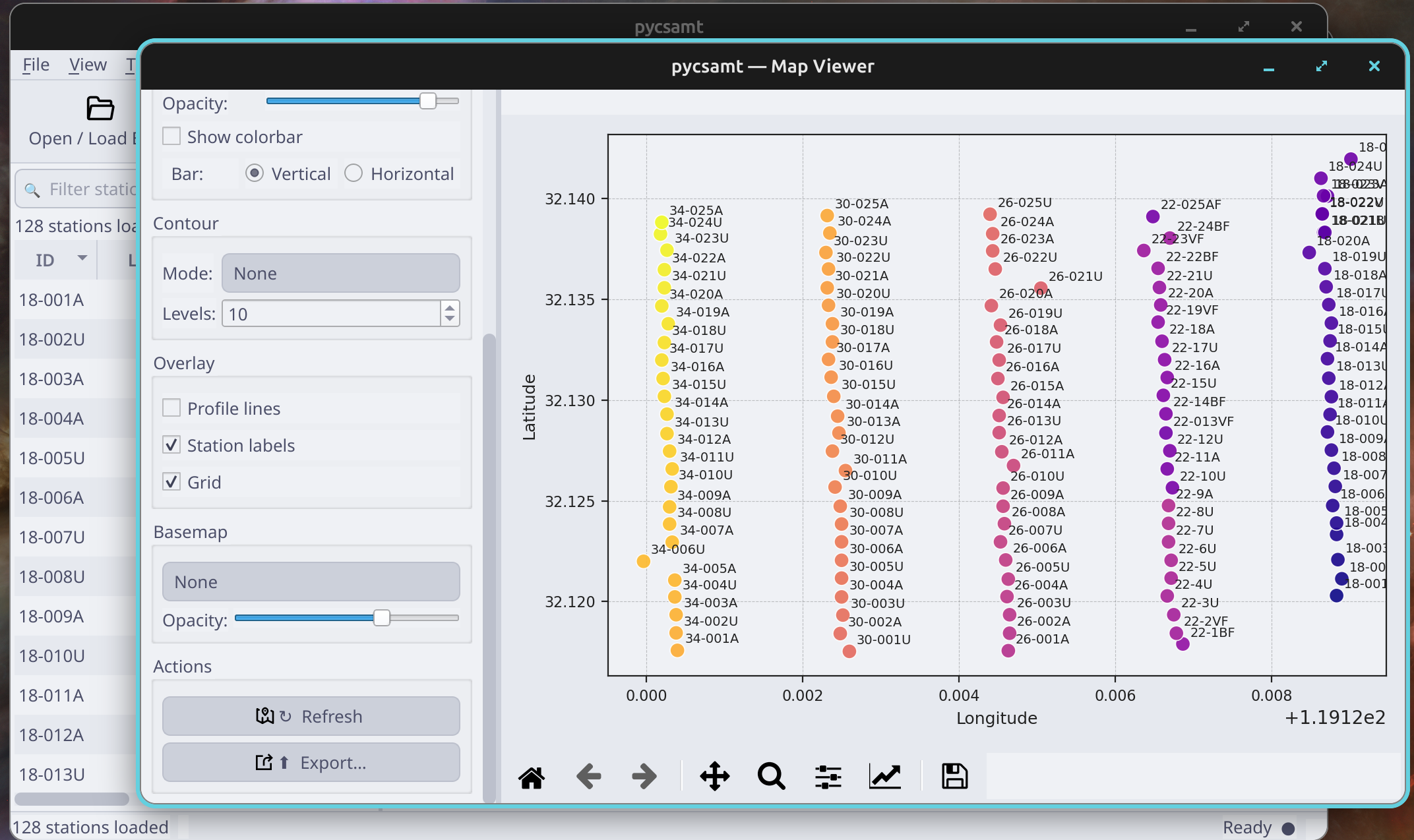
Station map in the pyCSAMT desktop map viewer — Station map with labels and grid enabled for a multi-line survey.#

Use the Map Type control to switch between:

Map type	Purpose
`Station`	Shows station locations, labels, profile lines, and coordinate sanity.
`Elevation`	Colours stations by elevation and can reveal topographic breaks.
`Depth`	Builds a depth-oriented view from loaded impedance data.
`Resistivity`	Maps apparent resistivity at a chosen frequency or period.

The left-side controls set display style, coordinate interpretation, and overlays. Refresh redraws the map with the current settings, and Export… writes the current figure through the shared export dialog.

Map Type Details#

The map type controls what quantity is drawn and which parameter groups become relevant.

Station: Draws station locations and labels. Use this view to verify station spacing, duplicated locations, reversed lines, missing coordinates, and line grouping. It is the safest view for the first check because it does not interpolate a geophysical attribute.
Elevation: Colours stations by elevation. Use it to detect missing elevation fields, unrealistic jumps, or a coordinate system mismatch. Elevation problems matter later because profile pseudosections and 2-D sections can include topography.
Depth: Produces a depth-oriented spatial view using the loaded impedance response and a target depth. The depth-to-period relation is a practical guide for inspection; it is not a substitute for inversion.
Resistivity: Maps apparent resistivity for the selected component at the selected frequency or period. Use this to find outlier stations and broad lateral contrasts before running correction or inversion workflows.

Coordinate System#

The map viewer assumes standard EDI station coordinates are geographic latitude and longitude. If the survey uses projected coordinates, change Input CRS before drawing:

Geographic (lat/lon) for normal EDI latitude/longitude metadata.
UTM Zone when station coordinates are in a UTM grid.
Custom EPSG for national grids or project-specific coordinate systems.

Choosing the right CRS matters before enabling basemap tiles or comparing line geometry to external maps. If the station cloud looks stretched, mirrored, or far from its expected area, check the CRS mode before interpreting any geophysical pattern.

Coordinate checks should happen before enabling basemap tiles. Basemaps can make a wrong CRS look obviously wrong, but they can also distract from the station metadata problem. First confirm that longitude/latitude or projected coordinates fall in the expected numeric range; then add external map context.

Frequency, Period, And Component#

Depth and resistivity maps use the loaded frequency axis. The viewer lets you work in either frequency or period:

choose Hz for frequency-domain inspection;
choose s (period) when thinking in skin-depth or profile-section terms;
use XY, YX, or Det to select the response component.

For depth maps, the Target depth control estimates the period associated with the requested depth from the loaded data. Treat this as an exploration aid rather than a formal inversion depth; use it to guide visual checks and then move to inversion or interpretation pages for modelling.

Component choice is part of the interpretation. XY and YX often carry the main off-diagonal MT/AMT response. Det is useful as a compact component when you want a quick scalar map, but it can hide directional differences that matter for strike, dimensionality, or static-shift checks.

Contours And Spatial Overlays#

Contours are useful only after the basic station geometry looks correct. The contour controls support line contours, filled contours, and filled contours with labels. Increase the number of levels when a smooth grid hides small structure; reduce it when interpolation artifacts dominate.

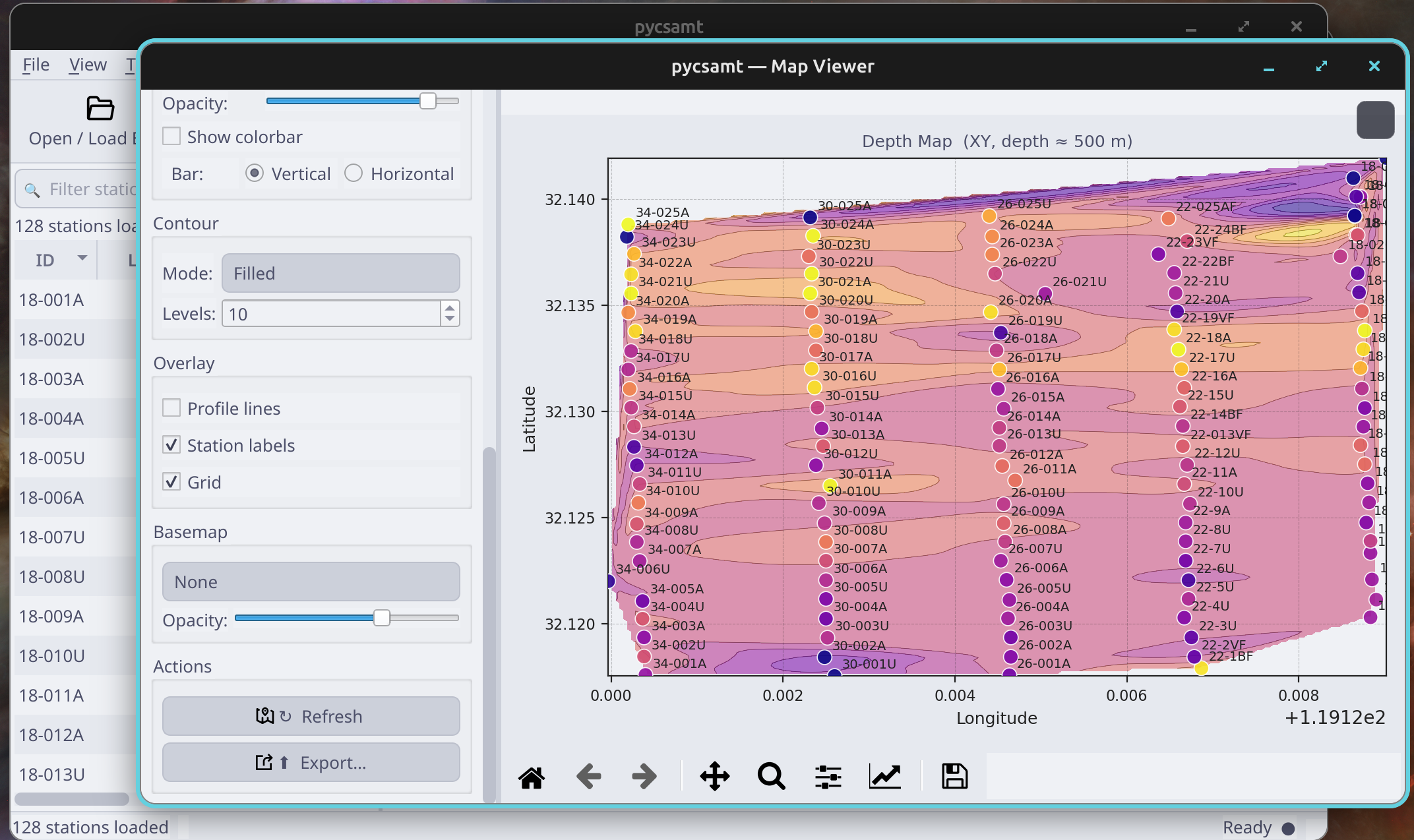
Filled contour depth map in the desktop map viewer — Depth-style map with filled contours, station labels, and the survey grid.#

Available overlays include:

Profile lines to connect stations by survey-line geometry.
Station labels for station-by-station checking.
Grid for quick coordinate inspection.
Basemap for optional tile context when contextily is available.

Basemap opacity is separate from marker opacity so you can keep map context visible without hiding the station markers. If contextily is not installed, basemap selection remains optional; the station and contour maps still work without web tiles.

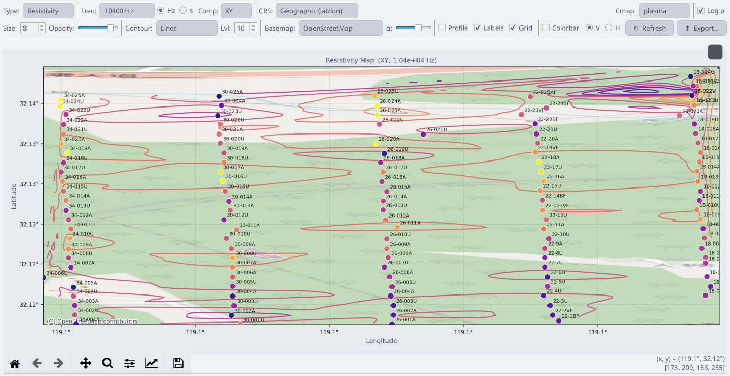
Map viewer with contour and display controls — The same map can be redrawn with different contour, label, grid, opacity, basemap, and export settings without reloading the survey.#

Contour Interpretation Rules#

Contours are an interpolation over station locations. They are useful for inspection, but they should be read with the station layout in mind:

do not interpret closed contour patches outside station coverage as mapped geology;
compare filled contours with the station markers before trusting gradients;
reduce contour levels when noise creates striping between adjacent stations;
use line contours when colour fill hides station-to-station jumps;
switch back to the station map if the contour shape is dominated by edge effects.

For sparse or irregular station spacing, a profile pseudosection is often more honest than a 2-D-looking filled map.

Selecting Stations From Maps#

Clicking a station in the map emits the same station selection used by the main window. This keeps the map, station table, station detail card, and profile viewer in sync. A practical inspection loop is:

Open the station map.
Click a station that looks spatially suspicious or geologically important.
Open the profile viewer for that station.
Check apparent resistivity, phase, tipper, and pseudosection context.
Return to the map and continue along the line.

This loop is especially useful before static-shift correction. A station that looks anomalous on the map should be checked in the profile viewer before it is treated as a real lateral feature.

Profile Viewer Overview#

The profile viewer is the station-response workbench. It starts with apparent resistivity and phase curves for the selected station, then exposes tabs for pseudosections, tipper, phase tensor, and 2-D section views.

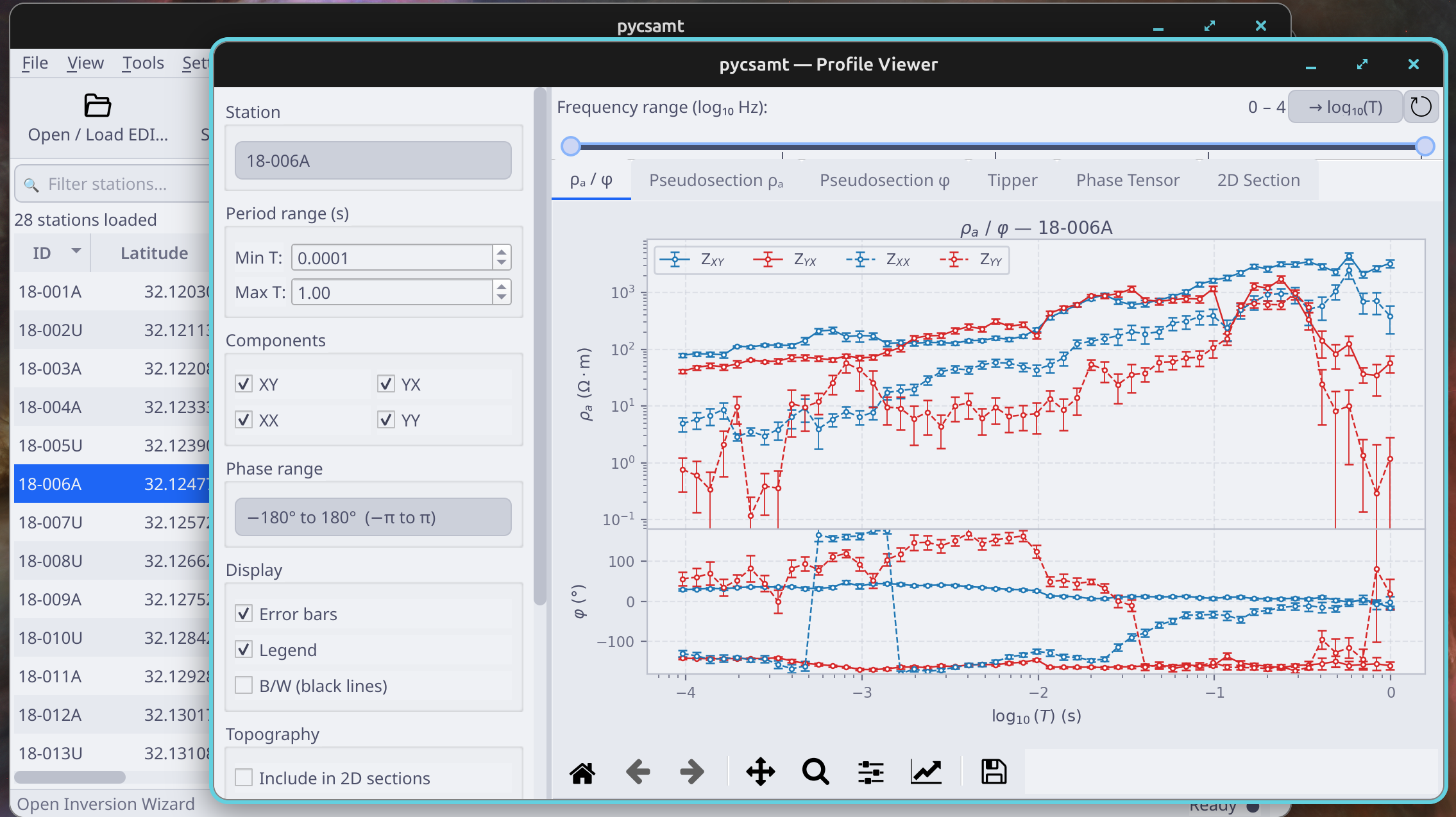
Profile viewer focused on one station with component, period, and display controls on the left.#

The station selector is searchable, which is useful for large surveys. The station selected in the main window is also propagated to the profile viewer.

Use the profile viewer to answer two different questions:

Is this station healthy? Check response curves, error bars, components, tipper availability, and phase behaviour.
Does this station make sense in the line? Compare the station with pseudosections, neighbouring stations, and phase-tensor or tipper patterns.

Response Controls#

Use the left-side controls to focus the response plot:

Period range limits the visible T interval.
Components toggles XY, YX, XX, and YY curves.
Phase range can be automatic or fixed to common intervals such as -180 to 180 degrees.
Error bars shows uncertainty where available.
Legend controls curve labels.
B/W (black lines) prepares monochrome-style plots for reports.

The quick toggle from frequency to log10(T) helps compare station curves with map depth settings and profile sections.

The default component set emphasizes XY and YX. Enable XX and YY when diagnosing diagonal leakage, distortion, rotation issues, or unexpected 3-D behaviour. If diagonal components dominate the response, move carefully before assuming a simple 2-D interpretation.

The phase range presets are not cosmetic only. They help distinguish wrapped or sign-convention issues from ordinary high-noise scatter. Use the automatic range for exploration, then fix the range when comparing multiple stations for reports.

Profile Tabs#

The profile viewer uses tabs to keep related diagnostics together:

Tab	Use it for
`rho_a / phi`	Per-station apparent resistivity and phase response curves.
`Pseudosection rho_a`	Along-line apparent resistivity structure by period.
`Pseudosection phi`	Along-line phase structure by period.
`Tipper`	Tipper magnitude/direction checks where tipper data exist.
`Phase Tensor`	Phase-tensor inspection for dimensionality and strike context.
`2D Section`	Section-style view for profile or inversion-oriented interpretation.

Topography can be included in pseudosections and 2-D sections when station elevation is available. The Exaggeration control changes terrain emphasis for visual inspection; it does not alter the underlying data.

Per-Tab Guidance#

rho_a / phi: Start here for every suspicious station. Look for discontinuities, noisy bands, component swaps, missing error bars, and phase values that sit outside the expected range.
Pseudosection rho_a: Use this to see whether an apparent resistivity anomaly is isolated to one station or continues along the line. Isolated vertical bands often deserve QC or static-shift attention before interpretation.
Pseudosection phi: Phase is less sensitive to static-shift amplitude effects than apparent resistivity. A resistivity anomaly without a phase counterpart should be checked carefully before treating it as structure.
Tipper: Tipper views require tipper data in the EDI files. Use them to inspect directional changes and possible lateral conductivity contrasts.
Phase Tensor: Use this before strike and dimensionality decisions. Strong beta changes, inconsistent ellipses, or abrupt rotations can signal 3-D effects or local data problems.
2D Section: This tab is the bridge to model and inversion review. It is most useful after an inversion result or section-style product has been loaded into the desktop session.

Publication View#

The profile viewer includes a Publication… action for a standalone multi-panel station view. Use it when a station has passed basic QC and you want a cleaner figure for a report or manuscript. Publication view does not change the active station data; it creates a separate figure-oriented view from the current station and display settings.

For publication-style figures:

fix the period and phase ranges before comparing stations;
decide whether colour or black-line mode is appropriate;
keep error bars visible unless the figure is explicitly schematic;
export figures from the viewer rather than taking screen captures.

Map And Profile Checks Before Processing#

Before running QC, correction, or inversion setup, use the two viewers as a short preflight:

station map: station count, line order, labels, coordinate range;
elevation map: missing elevations or unrealistic topographic jumps;
resistivity/depth map: obvious outliers or interpolation artifacts;
response curves: dead channels, swapped components, extreme error bars;
pseudosections: line continuity and frequency coverage;
phase tensor/tipper: directional behaviour that may affect strike or dimensionality assumptions.

The practical goal is to separate data-health problems from geological signals. If a feature appears in one station response but not in neighbouring stations or phase-sensitive views, investigate it through QC and correction before using it to guide inversion.

Hand-Off To Other Desktop Workflows#

The map and profile viewers do not perform correction or inversion themselves; they help you decide what to do next.

Use QC after the viewers reveal:

missing or sparse frequency coverage;
erratic error bars;
unusual component behaviour;
isolated stations that look unreliable.

Use Corrections after the viewers suggest:

static-shift-like amplitude offsets;
coordinate or elevation issues;
source-effect or rotation problems;
stations that need recomputed EDI output.

Use Forward or Inversion after:

station geometry and CRS are correct;
key components are usable;
pseudosections are continuous enough for modelling;
the interpretation target is clear.

Export Figures#

Both map and profile viewers use Export… for the current figure. The export dialog is shared with other desktop plots, so figure output uses the same desktop conventions as QC, correction, forward modelling, and interpretation windows.

Use exports for reports and documentation, but keep the project data and session file alongside exported figures so the view can be regenerated later.

Suggested filenames make later review easier:

L18_station_map.png
L18_resistivity_xy_10hz.png
L18_depth_500m_filled_contours.png
L18_station_18-006A_rhoa_phase.png
L18_phase_tensor_pseudosection.png

Common Issues#

No stations appear: Confirm that EDI files were loaded successfully and that the station table is populated. If the main table is empty, return to Loading Data And Sessions.
Stations plot in the wrong place: Check Input CRS. Standard EDI files are usually geographic latitude/longitude, but some project files may use UTM or another EPSG coordinate system.
Contours look blocky or misleading: Reduce contour levels, switch back to the station map, and confirm that station spacing supports interpolation. Sparse or uneven profiles should be interpreted with caution.
Basemap tiles do not appear: Basemap support requires optional geospatial dependencies and network tile access. The geophysical station maps still work without basemap tiles.
Profile tabs are empty: Select a station with valid impedance data and enough frequency samples. Some diagnostics, such as tipper views, require the corresponding data to exist in the loaded EDI files.