
4.6. Processing Pages#
The processing pages are where the web app turns a
loaded survey into scientific products: quality control,
corrections, advanced diagnostics, TDEM plots, pipeline runs,
forward model responses, inversions, interpretation
outputs, result reviews, and agent runs.
Each page is an interactive surface over the same
pycsamt.app.desktop.controllers used by the desktop app. A click in the
browser therefore delegates to the package rather than to a separate web-only
calculation, which is what lets a web session, a desktop session, and a Python
script reproduce the same result when they use the same inputs and options.
Most pages share a practical rhythm. Choose the survey subset, choose the operation, set the parameters, press the primary action, then inspect the plot, numbers, and run log. That rhythm is deliberate. Continuous recalculation would make large surveys feel busy and would also blur the record of what was actually run; explicit actions make the page state easier to audit.
4.6.2. Quality Control#
The Quality Control page is the first scientific checkpoint after loading data. It asks whether the response curves are dense enough, stable enough, and physically plausible enough to justify correction or modelling. In practical terms, QC reduces a response collection to interpretable metrics such as coverage, confidence, coherence, SNR, skew, dimensionality, and distortion indicators.
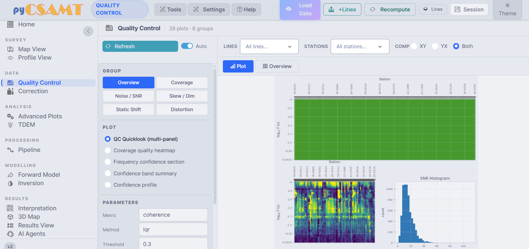
Quality Control. The group buttons separate survey coverage, noise, skew, static-shift, and distortion checks; the plotted panel is where isolated bad stations or frequency bands become visible before correction decisions are made.#
The plotted metrics usually start from a station-frequency response \(d_{i,j,c}\), where \(i\) indexes station, \(j\) frequency, and \(c\) component. A coverage-style diagnostic counts finite values in that grid, while confidence-style diagnostics combine noise, error bars, component consistency, and frequency continuity into a score. A simple threshold then acts as a mask, for example
where \(q_{i,j,c}\) is the chosen quality metric. The page does not ask you to trust the mask blindly: it puts the metric beside the survey structure, so a low-confidence band that crosses many stations reads differently from one isolated failing station.
Filters restrict the diagnostic to selected Lines, Stations, and component (
XY,YX, orBoth).Groups organise the checks into Overview, Coverage, Noise / SNR, Skew / Dim, Static Shift, and Distortion.
Plot list entries include QC Quicklook (multi-panel), Coverage quality heatmap, Frequency confidence section, Confidence band summary, and Confidence profile.
Parameters hold plot-specific choices such as metric, outlier method, threshold, and redraw behaviour.
QC should be read before correction. Sparse frequency coverage argues for frequency editing; coherent station-to-station offsets point toward static-shift review; erratic high-frequency scatter is more naturally a noise problem. That ordering keeps later corrections from becoming a cosmetic fix for data that should have been rejected or scoped more carefully.
4.6.3. Correction#
The Correction page applies pyCSAMT’s catalogue of corrections as a correction chain: 25 methods across 6 categories, previewed before they are committed, with per-step undo.
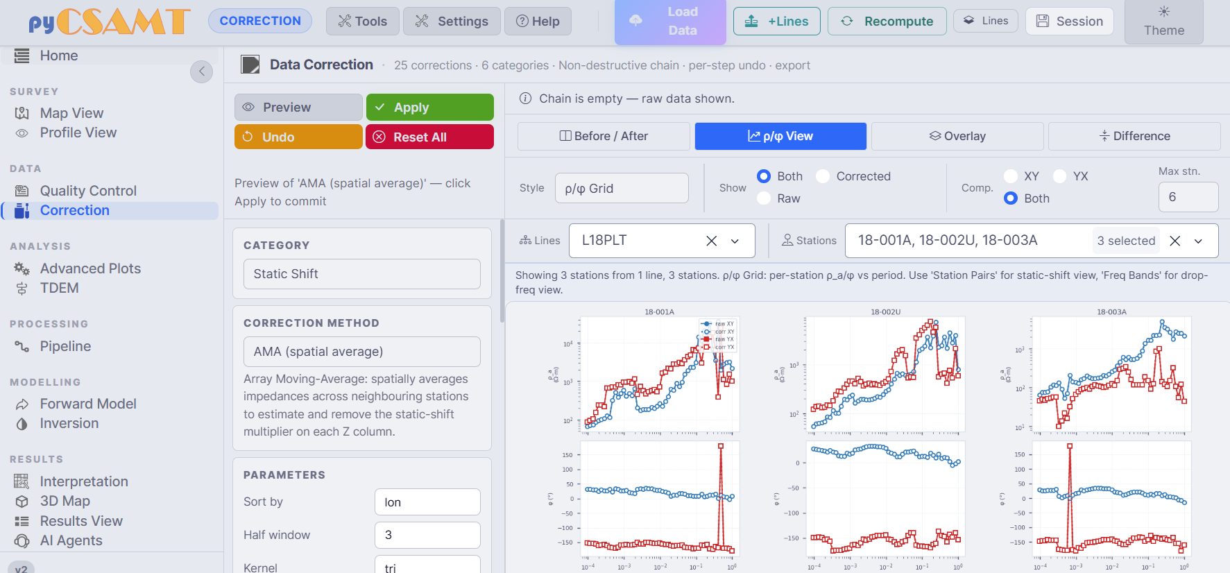
Correction. The preview panel compares raw and corrected responses before the operation is added to the chain; this is the point where a useful correction should reduce a systematic artefact without flattening real station-to-station structure.#
Mathematically, the page keeps the raw response \(d_0\) separate from the previewed response. A chain of accepted operations \(C_1,\ldots,C_k\) produces
Undo removes an operation from that ordered list; it does not try to reverse an edited raw file. That distinction matters most for static-shift correction, where apparent resistivity is rescaled by a station factor while phase should remain controlled by the inductive response. If \(g_i\) is the estimated static-shift factor for station \(i\), a typical correction is
The page’s Before / After, Overlay, and Difference views help check whether \(g_i\) removes a station offset while preserving curve shape. An AMA method, for example, estimates the shift from neighbouring stations, so it is strongest when the local station is offset but the regional trend is still shared across the line.
Category and Correction method choose the operation, such as Static Shift -> AMA (spatial average).
Parameters capture method-specific inputs, for example sort key, half-window, and kernel.
View modes compare raw and corrected responses as before/after panels, overlays, or differences.
Show and Comp choose raw/corrected/both and
XY/YX/both components across a limited station count.Actions separate Preview from Apply, with Undo and Reset All preserving a reversible review path.
Corrected EDIs are exported from this page; see Exports And Reproducibility. Treat them as derived products, not field originals.
4.6.4. Advanced Plots#
The Advanced Plots page gathers survey-scale diagnostics used for strike, dimensionality, and depth reasoning. These views are not later-stage decoration; they test whether the assumptions behind a 1-D, 2-D, or 3-D interpretation are defensible.
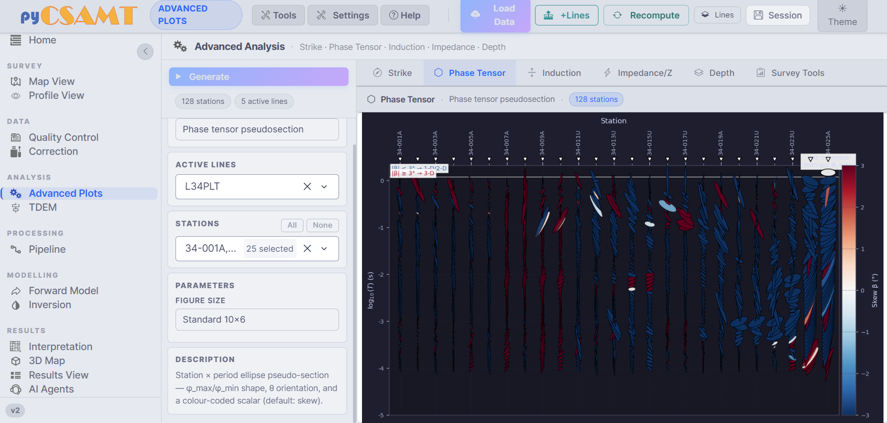
Advanced Plots on the Phase Tensor tab. The station-by-period ellipse section makes skew and orientation changes visible across the line, so a smooth 2-D assumption can be compared against the actual survey behaviour.#
The phase tensor is especially useful because it is insensitive to galvanic static shift. If \(\mathbf{Z}=\mathbf{X}+i\mathbf{Y}\) is the impedance tensor, the phase tensor is
Its ellipse orientation, ellipticity, and skew summarize how the response changes with period. Where ellipses rotate coherently along a profile, strike estimates are easier to defend; where skew is large or orientation changes abruptly, a simple 2-D rotation may be hiding 3-D structure.
Tabs expose Strike, Phase Tensor, Induction, Impedance/Z, Depth, and Survey Tools.
Active Lines and Stations scope the diagnostic to the chosen survey subset.
Parameters provide plot-specific inputs and figure-size presets.
Generate builds the selected diagnostic and shows a short description of the current plot.
These are whole-survey companions to Profile View. Use them when the question has moved from “is this station usable?” to “does the survey support the interpretation geometry I am about to use?”
4.6.5. TDEM#
The TDEM page handles time-domain electromagnetic data with its own folder browser and a fixed tab bar of plot categories. Unlike MT-style frequency responses, TDEM starts from a transient voltage or field decay after the transmitter current changes. The interpretation still depends on diffusion: early times mostly sample shallow structure, while later times reach deeper but lower-amplitude responses.
Tabs expose Decay / Rho, Survey Section, Map & Overview, and Dashboard.
Each tab provides plot choices, figure-size presets, and colour maps.
The folder browser points to a TDEM dataset before the selected plot is generated.
Read TDEM plots as time-domain diagnostics, not as another impedance plot. A smooth decay with coherent station variation can support section or map views; late-time oscillation, sign changes, or unstable apparent resistivity usually needs review before inversion or interpretation.
4.6.6. Processing Pipeline#
The Pipeline page turns the interactive processing sequence into an ordered, inspectable run. It is the repeatable counterpart to manually visiting QC, frequency editing, correction, strike analysis, rotation, and export pages. The important object is the sequence itself: if each step is represented as \(P_j\), then the processed survey after \(k\) steps is
The page records this chain in the progress track and output log, so the final export can be tied back to each operation rather than only to a final figure.
# |
Step |
What it does |
|---|---|---|
1 |
Load Data |
Use the loaded survey, or browse to a fresh EDI folder. |
2 |
QC Screening |
Drop low-confidence frequencies by threshold. |
3 |
Recover, trim, or mask frequencies by confidence and coverage. |
|
4 |
Static Shift Correction |
Apply a static-shift correction such as AMA. |
5 |
Denoise the impedance response while preserving interpretable shape. |
|
6 |
Strike Analysis |
Estimate geoelectric strike. |
7 |
Rotate impedance components to the strike frame. |
|
8 |
Export |
Write processed EDIs and products to an export folder. |
Run Step executes only the current step; Run All executes the remaining
steps in order; Skip advances without running; and Reset returns to the
start. For each step you choose a method and see a description, while the
Log, Preview, and Status result tabs show what happened. A message
such as ERROR: SVD did not converge is not just a software complaint; it
means the selected method and data subset did not produce a stable solve, so
parameters or prior QC decisions should be revisited before export.
4.6.7. Forward Modelling#
The Forward Model page computes synthetic responses in 1-D, 2-D, and 3-D. It answers the forward question: if an earth model \(m\) is assumed, what data should the survey measure?
where \(F\) is the forward operator. The page exposes the model geometry, background resistivity, frequency sampling, and station layout because all of them affect \(d_{pred}\).
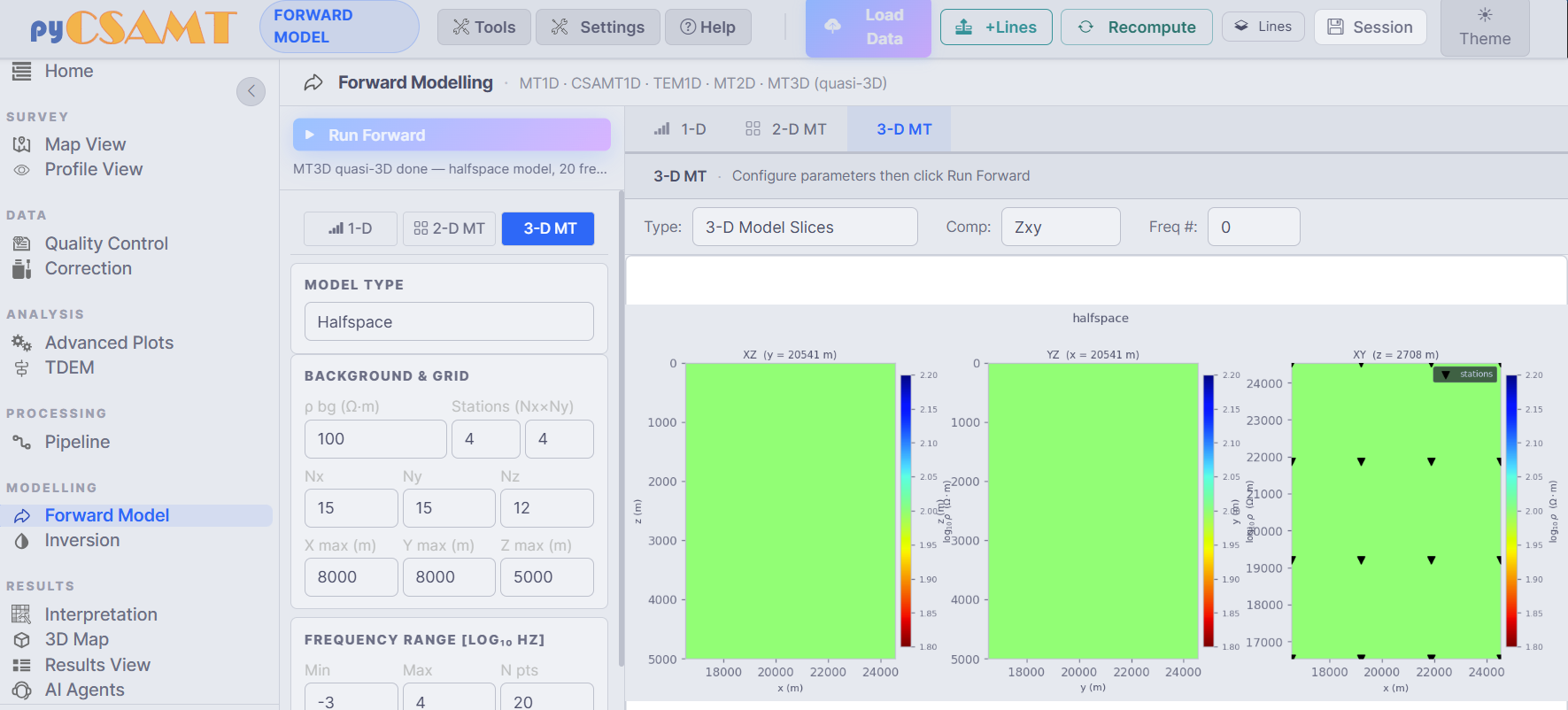
Forward Model on the 3-D MT tab. The model slices and response controls make the modelling assumptions visible before the synthetic response is used for intuition, testing, or AI-inversion training.#
Tabs separate 1-D, 2-D MT, and 3-D MT (quasi-3D) modelling.
Model Type chooses a halfspace, layered model, or preset structure.
Background & Grid define background resistivity, station layout, grid dimensions (
Nx x Ny x Nz), and extents.Frequency Range defines
log10(Hz)min/max and the number of sampled frequencies.Run Forward computes the response and draws the model and selected component/frequency response.
Use this page to build intuition before inversion. A conductive target, resistive basement, or shallow layer has a recognisable response only under the assumptions used to generate it; changing frequency range, station spacing, or dimensionality changes the synthetic evidence.
4.6.8. Inversion#
The Inversion page works in the opposite direction: it estimates a model from observed or synthetic data. All inversion families on the page are trying to reduce some version of data mismatch while keeping the model plausible, but they do it with different machinery.
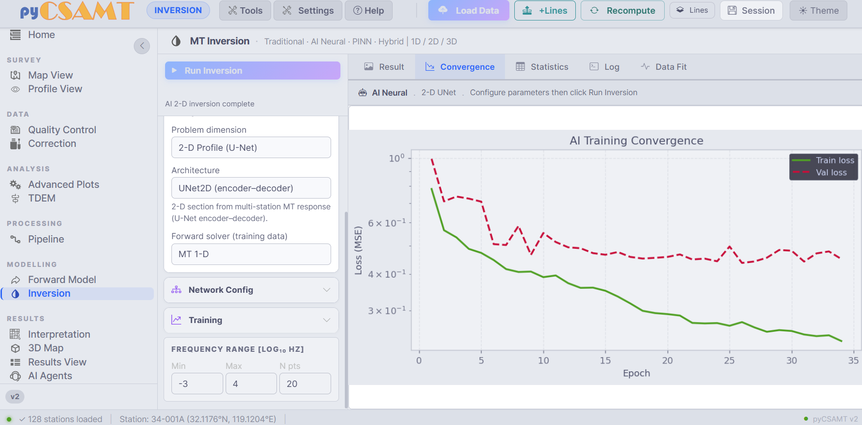
Inversion configured for a 2-D AI-neural U-Net run. The convergence curve shows optimization progress; the model is not accepted until its response fit and residual pattern are also reviewed.#
A traditional inversion minimizes an objective such as
where \(W_d\) weights data uncertainty, \(W_m\) controls roughness or departure from a reference model, and \(\lambda\) balances fit against regularity. An AI inversion learns an inverse mapping from training examples and must be checked against its training distribution and feature contract. A PINN adds a physics residual to the neural loss, and a hybrid inversion uses an AI estimate together with a physics-based refinement.
Problem dimension selects a 1-D, 2-D, or 3-D formulation, such as 2-D Profile (U-Net).
Architecture chooses the network or solver, for example UNet2D (encoder-decoder).
Forward solver (training data) declares the physics used to generate training responses.
Network Config and Training hold architecture and optimization settings.
Frequency Range fixes the band used in the inversion.
Result tabs separate Result, Convergence, Statistics, Log, and Data Fit.
Run Inversion starts the run.
Read training convergence as an optimization diagnostic, not as final geological proof. A smooth loss curve means the optimiser found a lower-loss solution under the declared setup. The next question is data fit: do the predicted apparent resistivity and phase match observations within the assigned errors, and are residuals random rather than systematic?
4.6.9. Results View#
The Results View page, labelled Inversion Results Viewer in the app, browses, inspects, and exports outputs from external solvers: ModEM, Occam2D, and MARE2DEM.
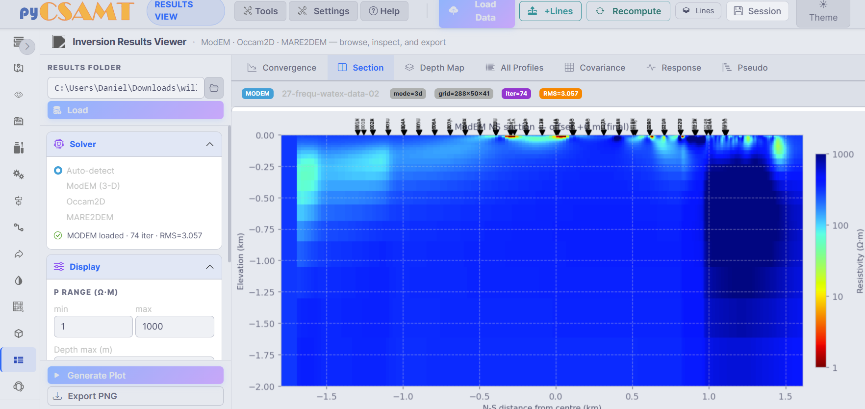
Results View on the Section tab. The resistivity section is easier to read beside the solver metadata because iteration count, RMS, grid, and loaded solver all affect how much confidence the section deserves.#
Results Folder points to a solver output folder and Load imports it.
Solver can auto-detect the engine or force ModEM (3-D), Occam2D, or MARE2DEM.
Tabs expose Convergence, Section, Depth Map, All Profiles, Covariance, Response, and Pseudo.
Display controls resistivity range and maximum depth.
Generate Plot redraws with the current settings; Export PNG saves the figure.
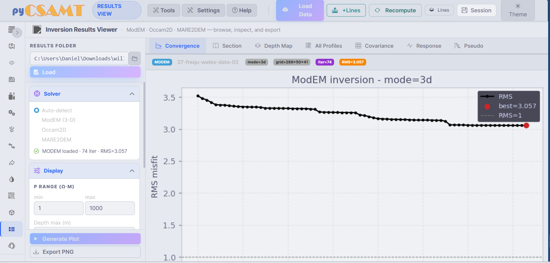
The Convergence tab shows RMS misfit versus iteration. A falling curve toward the RMS=1 target suggests the model is fitting within assigned uncertainty; a stalled or rising curve usually points to the data errors, starting model, regularization, or physics assumptions.#
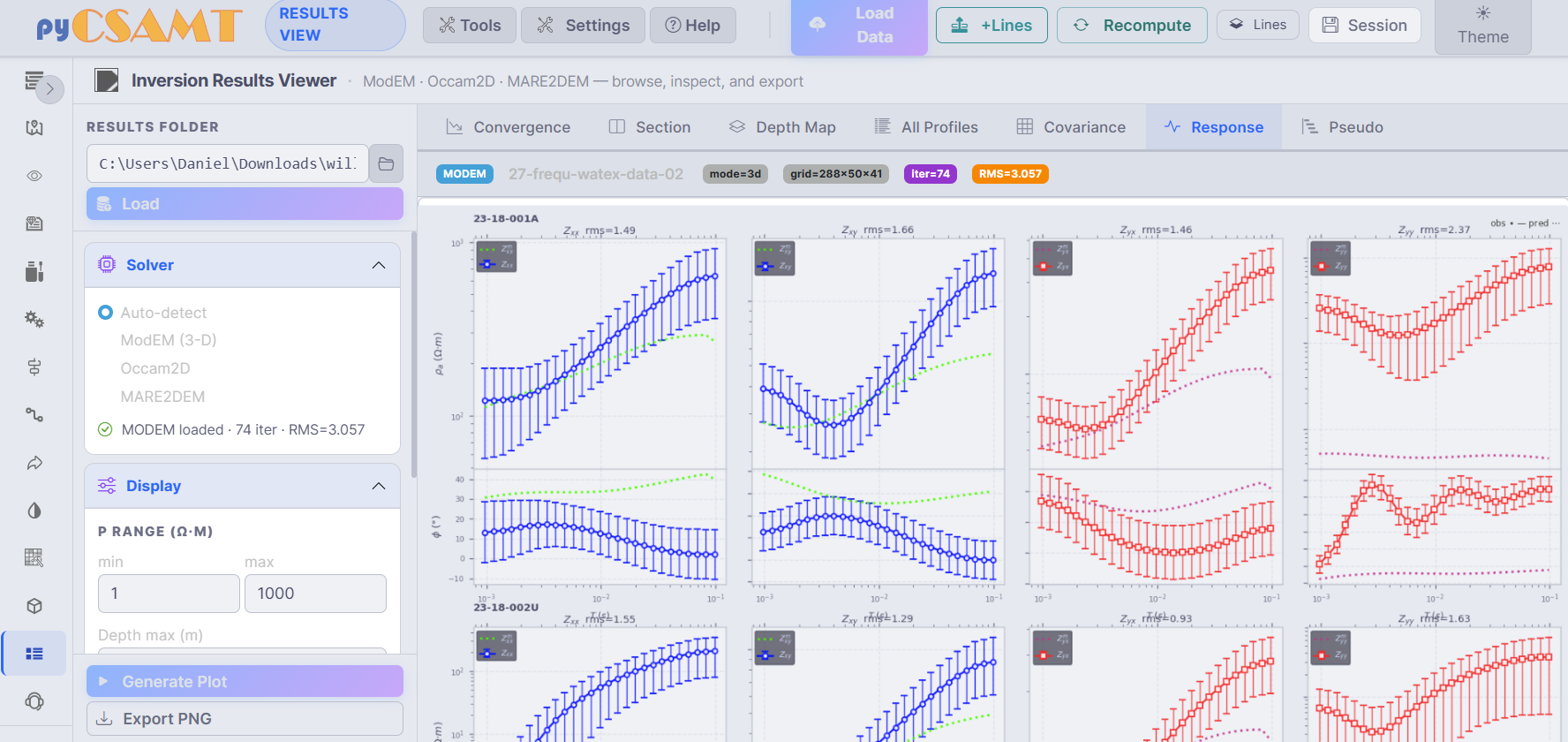
The Response tab compares observed and predicted apparent resistivity and phase. Station-level RMS values are useful, but the curve shapes matter: repeated residual structure across frequency or component is stronger evidence of model mismatch than one isolated noisy point.#
The results viewer is where visual interpretation and numerical fit meet. A section can look geologically attractive while still fitting one mode poorly; the convergence and response tabs are there to keep the story honest.
4.6.10. Interpretation#
The Interpretation page turns processed data and models into geological, hydrological, diagnostic, and export products. It contains 42 workflows across 9 categories, but the working logic remains the same: choose the evidence source, choose the analysis, set display or export options, and generate a traceable product.
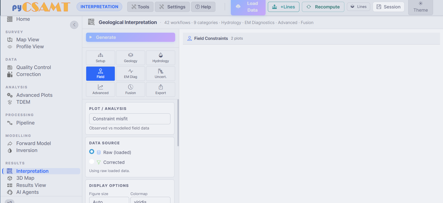
Interpretation. The page keeps the data source and display controls beside the generated view so the reader can tell whether an interpretation was made from raw, corrected, modelled, or exported evidence.#
Categories include Setup, Geology, Hydrology, Field, EM Diag, Uncert., Advanced, Fusion, and Export.
Plot / Analysis chooses the workflow, for example Constraint misfit - observed vs modelled field data.
Data source selects Raw (loaded) or Corrected.
Display options control figure size, colour map, and workflow-specific parameters.
Generate builds the product; Export saves interpretation outputs.
Interpretation products should remain tied to their inputs. When a workflow uses a calibrated model, borehole constraint, or uncertainty setting, the exported product belongs with that evidence and with provenance manifest; otherwise a reviewer cannot tell whether a geological label came from data, model calibration, or presentation choice.
4.6.11. AI Agents#
The AI Agents page exposes pyCSAMT’s agents in two modes: a direct Agent Runner and a conversational Chat assistant over the loaded survey. Agents do not replace the processing pages; they orchestrate the same operations and report the result as a run history, log, summary, and optional figure.
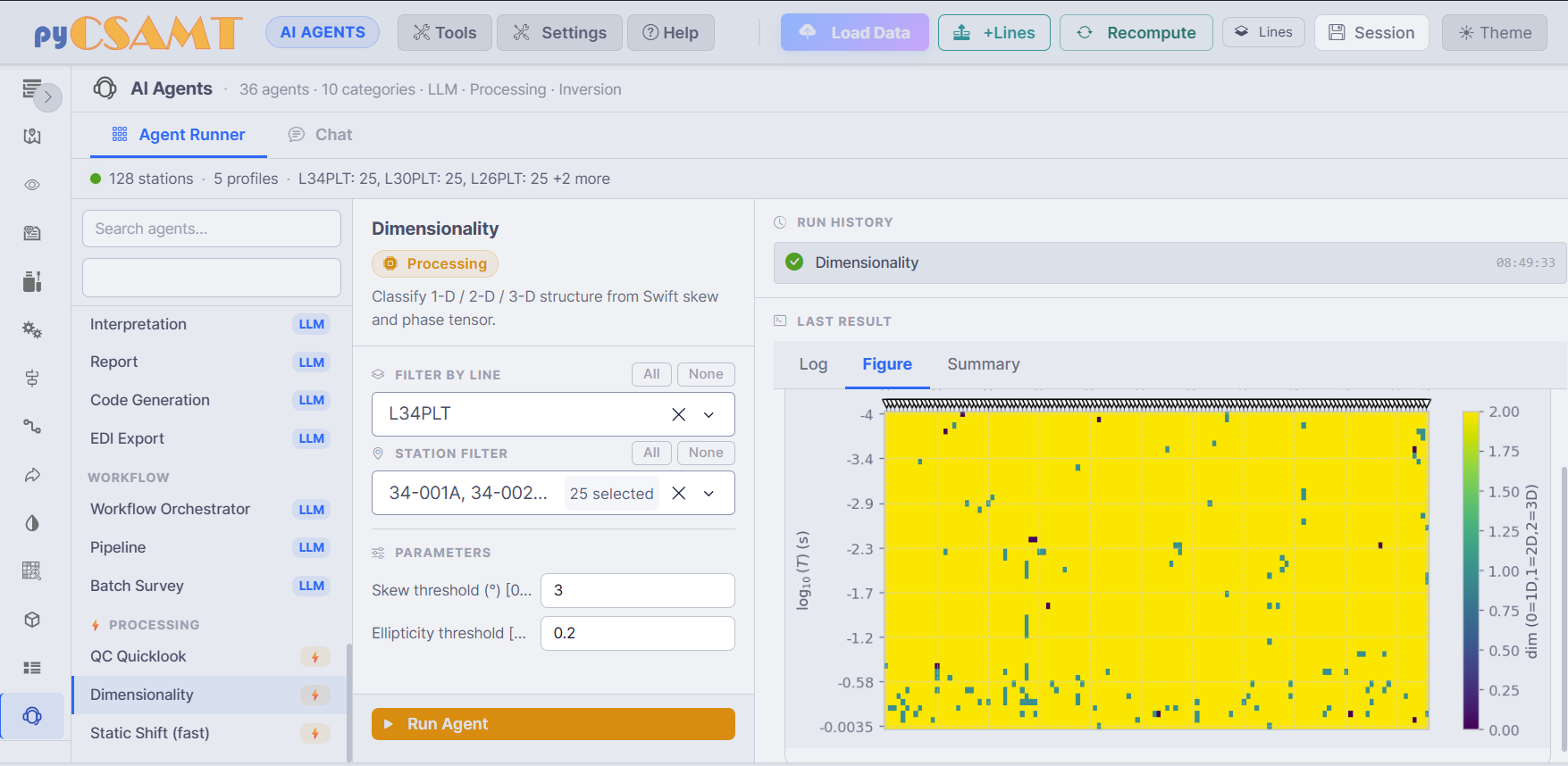
Agent Runner. Search and pick an agent, scope it by line and station, set parameters, and run it; the right-hand panel keeps the latest log, figure, and summary together.#
The agent list is grouped into LLM agents, workflow agents, and processing agents. Selecting an Agent reveals its description, line and station filters, and parameters. After Run Agent, the run history records what ran and the last-result panel shows the evidence the agent produced. A dimensionality agent, for example, should be judged against the same skew, phase-tensor, and impedance evidence you would inspect manually.
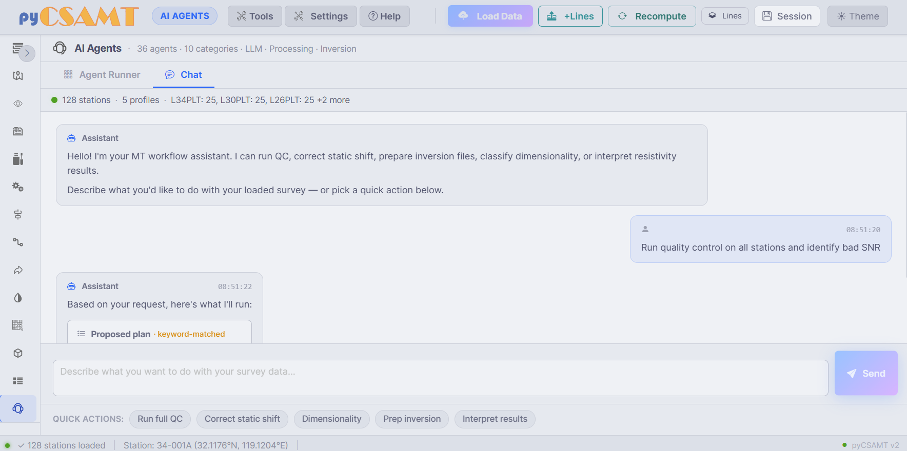
The Chat tab. Natural-language requests are converted into runnable plans; quick actions cover common QC, correction, dimensionality, inversion-prep, and interpretation workflows.#
Type a request such as Run quality control on all stations and identify bad
SNR and the assistant proposes a runnable plan. LLM-backed features need an
LLM provider and API key configured in the Settings drawer; the
non-LLM processing agents can still run deterministic package workflows when
they do not need language-model reasoning. For a dedicated, full-screen
conversational surface, use Agent Master.
4.6.12. Tools#
The Tools menu on the command bar collects standalone utilities that open in their own drawer. They are independent of the current page but still read from the active survey.
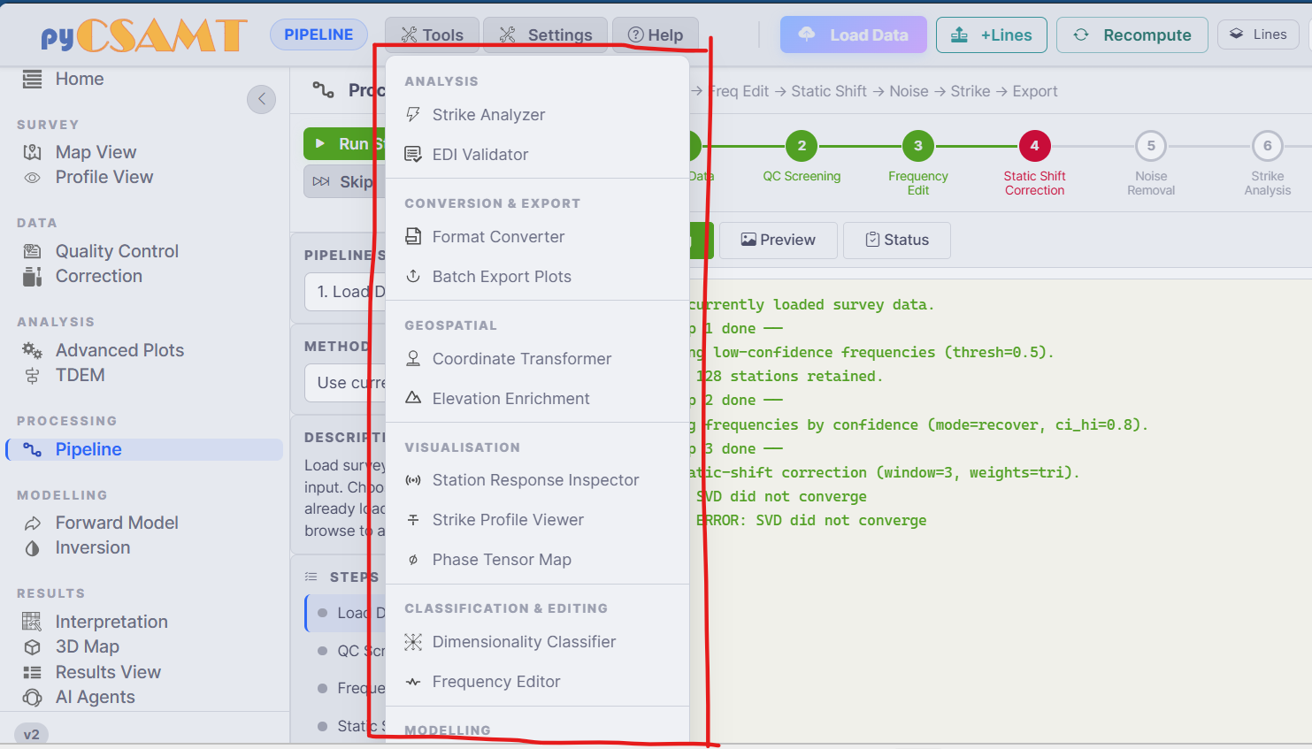
The Tools menu groups focused utilities by purpose, so quick validation, conversion, geospatial, and visualisation tasks can be run without changing the main processing page.#
Group |
Tools |
|---|---|
Analysis |
Strike Analyzer, EDI Validator |
Conversion & Export |
Format Converter, Batch Export Plots |
Geospatial |
Coordinate Transformer, Elevation Enrichment |
Visualisation |
Station Response Inspector, Strike Profile Viewer, Phase Tensor Map |
Classification & Editing |
Dimensionality Classifier, Frequency Editor |
Modelling |
Modelling utilities |
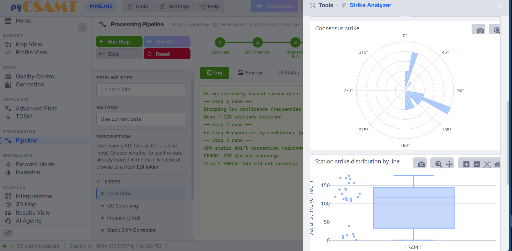
The Strike Analyzer tool compares consensus strike with per-line distributions. Agreement across lines supports a shared rotation; strong line-to-line disagreement is a warning to inspect dimensionality before applying one strike angle everywhere.#
The Batch Export Plots tool is the fastest way to export many figures at once; see Exports And Reproducibility.
4.6.13. How Pages Delegate To The Package#
None of these pages implement science of their own. A control change updates a
Dash store, and the primary-action callback calls the matching
pycsamt.app.desktop.controllers function. In reproducibility terms, the
browser state is only the interface layer; the scientific record is the input
survey, selected mask, method, parameters, package version, output files, and
run log. This is why a survey processed in the web app can be picked up
unchanged in the desktop app or in a script.
4.6.14. Next Steps#
Exports And Reproducibility – save figures, corrected EDIs, and inversion products.
Maps And Profiles – the spatial views that precede processing.
Troubleshooting – when a page is blank, a run fails, or an agent errors.