Views And Controls#

MapView organises everything around two views, switched from the left rail: Map (2-D) and 3-D. Both read the same loaded survey and respect the line picker, so switching views never changes what is selected — only how it is drawn.

The Shell#

Every view shares the same frame:

Top bar — the app title, Load lines and Add line, a live N stations · M line(s) status, then Session, Export, a theme toggle, Help, Sites, and the inspector-panel toggle.
Left panel — the Lines picker (an All chip plus one per line) and the Stations list, each row with an eye toggle to show or hide a station.
Canvas — the current view, with a view-specific toolbar along the top.
Inspector — a right-hand panel of controls for the current view; it can be collapsed from the top bar to widen the canvas.

Map View#

The Map view is the 2-D basemap picture of the survey.

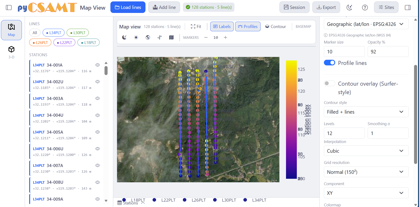
The Map view: the Lines/Stations panel on the left, the basemap canvas with the colour scale, and the inspector on the right.#

Canvas toolbar

Fit re-frames the map to the survey extent.
Labels toggles station labels.
Profiles toggles the profile lines connecting each line’s stations.
Contour toggles the Surfer-style contour overlay.
Basemap selects a tile style — dark, light, satellite, topographic, or street.
Markers steps the marker size up or down.

Inspector controls

Control	Effect
Colour by	The field drawn on markers: Station index, Elevation, App. resistivity, Phase, or Skin depth.
Frequency	The frequency at which resistivity/phase/skin-depth fields are evaluated (a slider).
Basemap	The tile provider (for example Open Street Map).
Coordinate system	How station coordinates are interpreted — Geographic (lat/lon · EPSG:4326), a UTM zone, or a custom EPSG.
Marker size / Opacity %	Marker appearance.
Profile lines	Draw the per-line connectors.
Contour overlay (Surfer-style)	Draped contours, with Contour style (filled, lines, or both), Levels, Smoothing σ, Interpolation (for example cubic), Grid resolution, Component, and Colormap.

Tip

Set the Coordinate system correctly before reading position or contours. Standard EDI files are geographic latitude/longitude; project files may use a UTM zone or a custom EPSG code.

The Contour Overlay#

Turning on Contour drapes a Surfer-style interpolated surface over the basemap — useful for a quick lateral sense of a field before moving to 3-D.

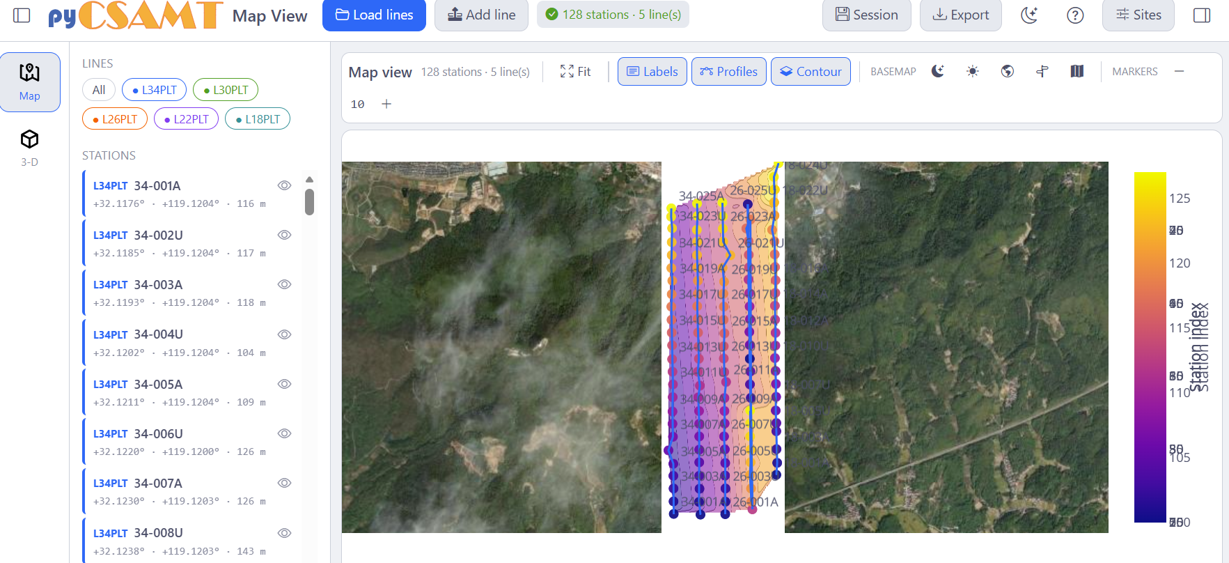
MapView Map view with a filled contour overlay over the satellite basemap — A filled-and-lines contour overlay of the station-index field, draped over the survey lines. Read contours with the station layout in mind — they are an interpolation, not mapped geology.#

Basemaps#

The basemap can be satellite imagery, a light or dark canvas, a topographic tileset, or a street map.

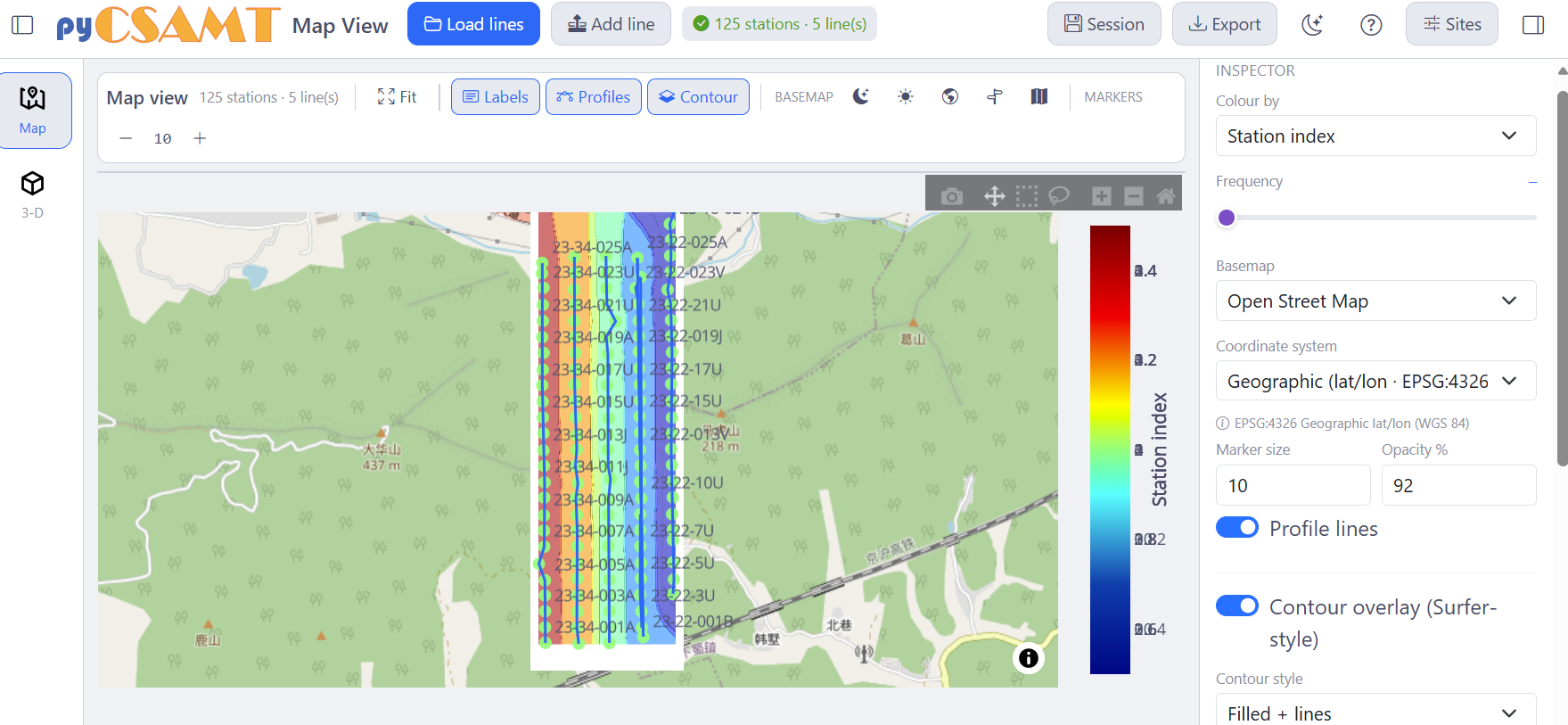
MapView Map view on an Open Street Map basemap with the inspector open — The same survey on an **Open Street Map** basemap, with the full inspector showing the colour field, frequency, basemap, coordinate system, marker, and contour controls. The Plotly modebar (top-right of the canvas) gives pan, zoom, box/lasso select, and a PNG snapshot.#

3-D View#

The 3-D view renders the survey’s resistivity as an interactive scene. Switch to it with 3-D in the left rail.

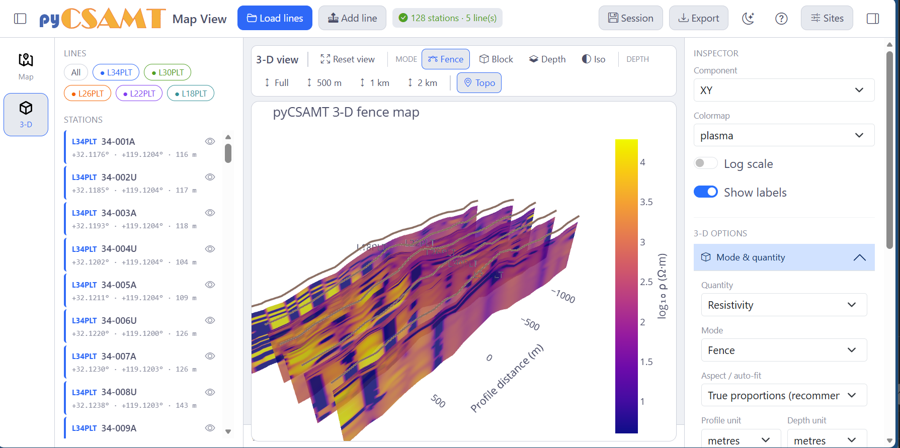
MapView 3-D fence map with draped topography — The 3-D view in **Fence** mode with topography: one vertical resistivity panel per survey line, a terrain surface draped from station elevations, and the log₁₀ ρ colour bar. The inspector’s **3-D options** accordion holds mode, depth, resistivity, geometry, topography, station, and appearance controls.#

Canvas toolbar

Reset view returns the camera to its default framing.
Mode — Fence, Block, Depth slices, or Iso surface.
Depth — quick vertical windows: Full, 500 m, 1 km, 2 km.
Topo toggles the draped topography.

Render modes

Mode	What it draws
Fence	A vertical resistivity panel along each survey line — the closest 3-D analogue of a pseudosection, seen in place.
Block	A filled semi-transparent volume interpolated across the survey.
Depth	Horizontal depth slices through the volume.
Iso	Iso-surfaces at chosen resistivity levels — good for isolating discrete bodies.

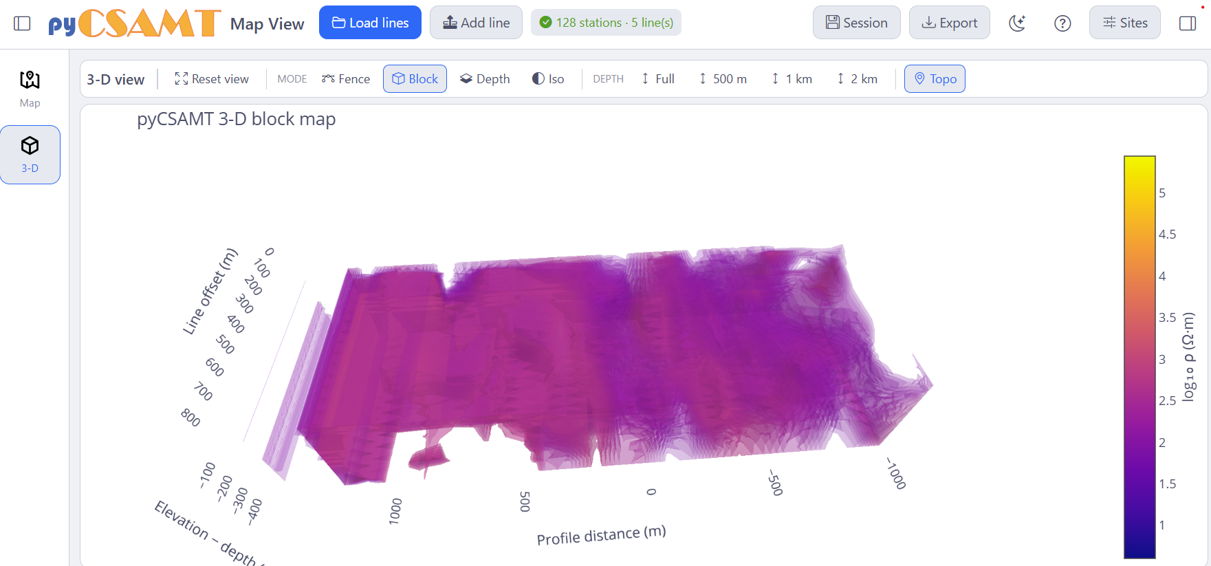
MapView 3-D block map — **Block** mode renders the survey as a filled, semi-transparent resistivity volume; **Reset view**, the mode buttons, the depth window, and **Topo** are all on the canvas toolbar.#

Inspector — 3-D options

The 3-D inspector groups its controls into an accordion:

Mode & quantity — the Quantity (Resistivity), the render Mode, the Aspect / auto-fit (True proportions is recommended), and the Profile and Depth units.
Depth filter — the Quick window (Full / 500 m / 1 km / 2 km), an explicit Depth window (m), the number of Depth slices, and the number of Iso-surfaces.
Resistivity range — the ρ visibility band and window (see below).
Geometry, Topography, Stations (3-D), and Appearance — scene geometry, terrain, in-scene station markers/labels, and styling.

Above the accordion, Component, Colormap, Log scale, and Show labels control the colour axis and labelling.

Isolating Conductive Or Resistive Structure#

The Resistivity range section is one of MapView’s most useful 3-D tools. The ρ visibility band (All, Conduct., Mid, Resist.) with an explicit ρ visibility (Ω·m) window fades everything outside the chosen band in Block and Iso-surface modes (and hides individual cells outside it in Fence and Depth modes), so you can look at just the conductive or just the resistive part of the volume.

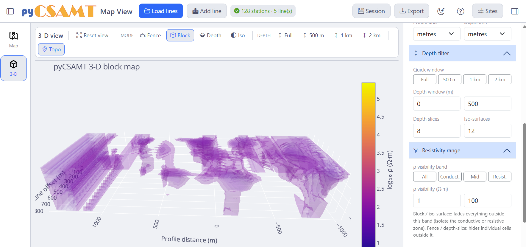
MapView 3-D block map showing only the conductive band — Block mode with the **Conduct.** band (ρ ≈ 1–100 Ω·m): only the conductive structure remains visible.#

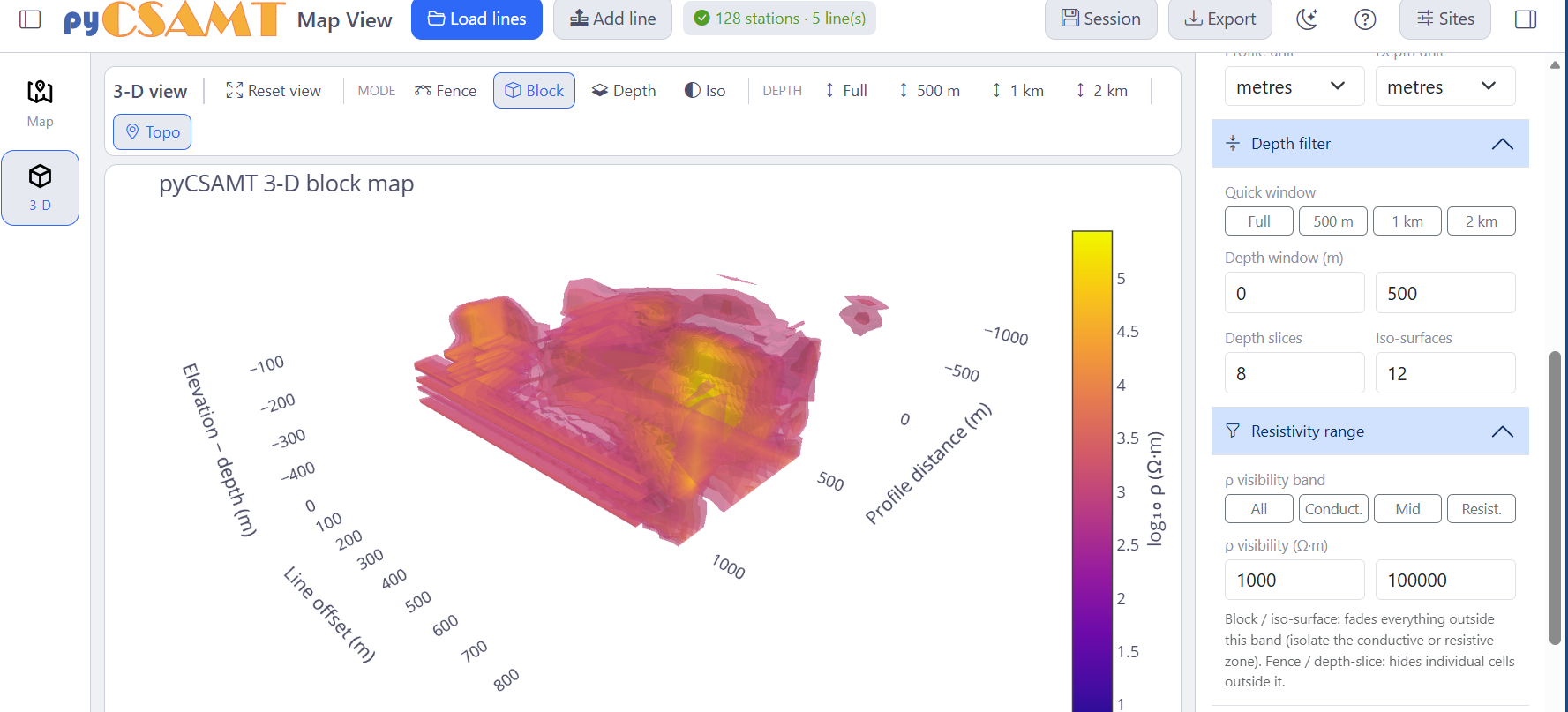
MapView 3-D block map showing only the resistive band — The same scene with the **Resist.** band (ρ ≈ 1000–100000 Ω·m): now only the resistive bodies show. Switching the band is the fastest way to separate the two.#

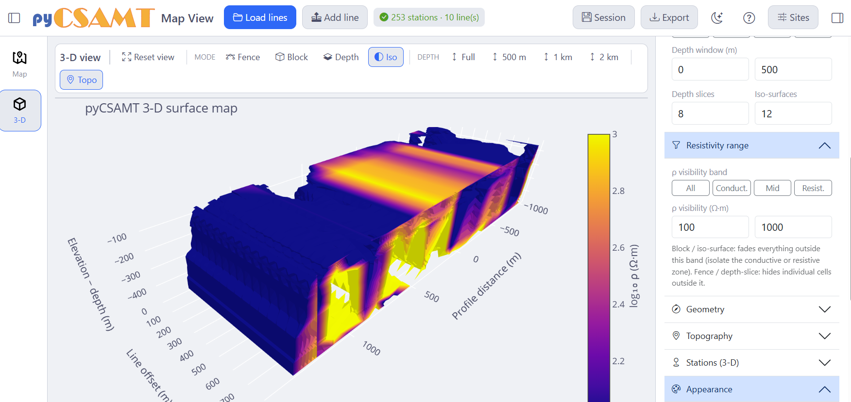
MapView 3-D iso-surface map with depth and resistivity controls — **Iso** mode with the **Depth filter** and **Resistivity range** panels open: depth window, depth slices, and iso-surface count on the left of the panel; ρ visibility band and window below.#

Inversion Results In 3-D#

When you import a ModEM 3-D inversion result (see Loading Data And Sessions), the same 3-D view renders the inverted resistivity model instead of an interpolation of the survey response — one panel per detected line, in the survey’s own scene.

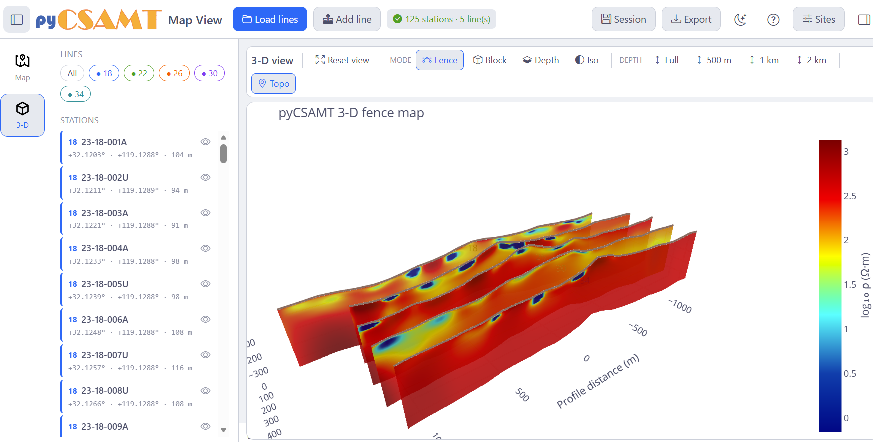
MapView 3-D fence map of an imported ModEM inversion result — A ModEM inversion result shown as fence panels: conductive pockets (blue) embedded in a resistive background (red), sliced to one panel per line, with the depth window set to 500 m.#

Every 3-D control applies to the imported model — modes, depth windows, the resistivity band, and topography. Iso-surface mode with hover read-outs is especially useful for locating and measuring discrete bodies in the inverted volume:

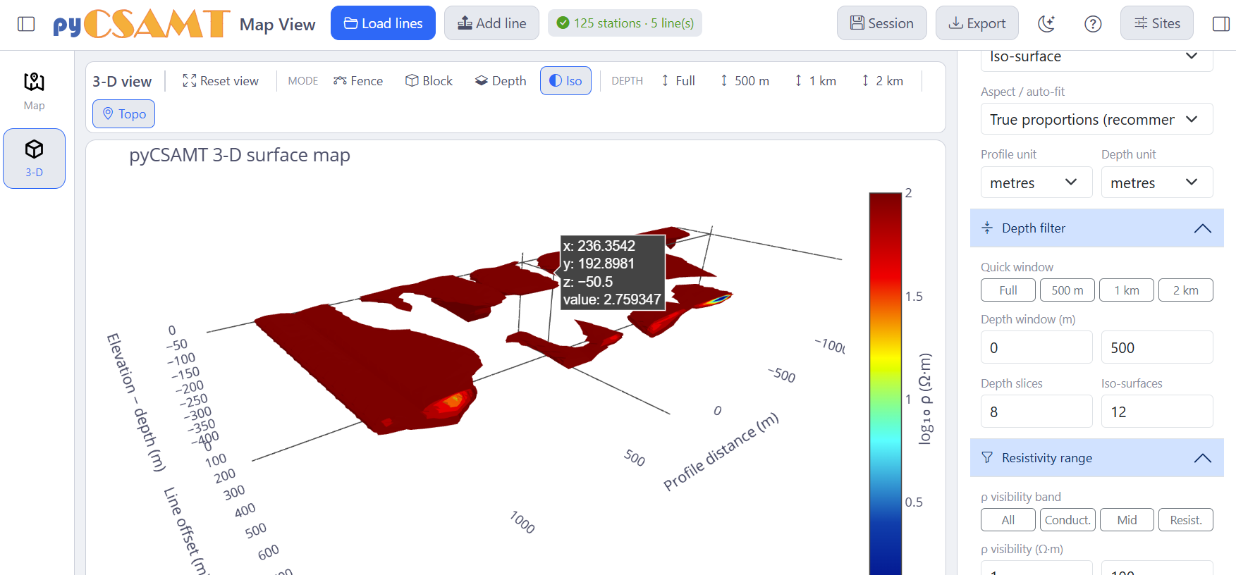
MapView 3-D iso-surface of an inversion result with a hover read-out — Iso-surfaces of the inverted model, with a hover tooltip reporting the position and log₁₀ ρ value at a point — the direct way to interrogate a body in the model.#

Note

The 3-D scene is WebGL. If the Map view works but the 3-D canvas stays blank, see Troubleshooting.