3.4. Workspace And Navigation#

The pyCSAMT desktop workspace is deliberately lean. The main window keeps the loaded survey visible, while maps, profiles, QC, corrections, modelling, and agents open as independent panel windows. This lets you keep the station list anchored on one screen and move the scientific views around it.

3.4.1. Why The Workspace Is Split Into Panels#

Desktop processing is an evidence-building workflow. A user often needs to compare a station table, a response curve, a map, a QC metric, and a correction preview before deciding what to do. Separate panels make that comparison possible without forcing every view into one crowded tab stack.

The main window should remain the reference point for the active survey:

it shows which station is selected;
it exposes the current data-state label;
it records messages in the log dock;
it keeps the toolbar and menus available while scientific panels are open.

Use the floating panels as working views around that reference point. When a plot looks surprising, return to the station list, detail card, status bar, and log before changing the data state.

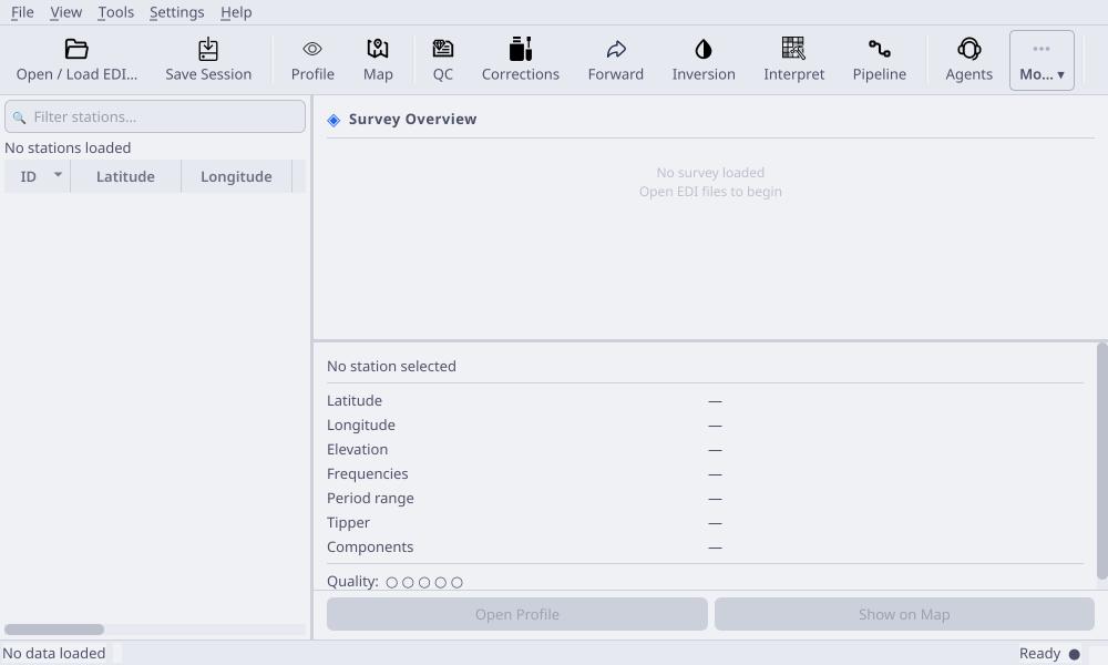
pyCSAMT desktop main workspace after launch — The main workspace is the command centre: toolbar at the top, station list on the left, survey and station summaries on the right, and a compact log dock at the bottom.#

3.4.2. Main Window Regions#

The main window has four persistent regions:

Toolbar – one-click access to loading, saving, viewers, processing, and export tools.
Station list – searchable table of loaded stations.
Survey overview and station detail – summary cards for the whole line and the currently selected station.
Log and status areas – loading messages, processing messages, progress, and the current data-state label.

The main window owns the active survey. When data are loaded or replaced by a committed correction, the station list and open panel windows are refreshed from that active survey.

3.4.3. Orientation After Loading#

After a survey loads, pause for a short orientation pass before opening many tools. The goal is to answer, “What data state am I looking at right now?”

Read the status bar and confirm that data are loaded.
Check the survey overview for station count, frequency range, and basic metadata.
Select one station and read the station detail card.
Open Profile for that station and confirm curves render.
Open Map and confirm the station cloud is plausible.
Return to the main window and save the session if the workspace is arranged correctly.

This small habit prevents a common desktop mistake: interpreting a map, profile, or QC figure without being sure whether the active survey is raw, corrected, recomputed, or reloaded from a different folder.

3.4.4. Station List#

The station list is the primary navigation surface after loading EDI files. Use the search field above the table to filter station IDs while keeping the loaded survey unchanged. Selecting a station updates the detail card and also notifies open profile/map windows.

Normal station-list workflow:

Load one survey line or a focused folder of EDI files.
Use the search field to isolate a station or station prefix.
Select a row to inspect its metadata in the detail card.
Open Profile or Map from the toolbar to inspect the selected station in context.
Clear the search text before checking line-wide coverage or profile trends.

Filtering is only a view operation. It does not remove stations from the active Sites object and it does not affect export or processing windows.

Use the station list for navigation, not data editing. If a station needs to be removed, flagged, corrected, or excluded from inversion, make that decision in the relevant QC, correction, pipeline, or inversion workflow so the choice is recorded. A search filter only changes what is visible on screen.

3.4.5. Survey Overview#

The survey overview card summarizes the loaded data set. Use it immediately after loading to confirm that the number of stations, file set, and frequency coverage look plausible before opening heavier processing tools.

If the overview does not match the line you intended to load, stop and reload the data. It is better to fix a folder-selection mistake before QC, maps, or corrections start producing convincing figures from the wrong input.

Use the overview as a gate before deeper work:

station count should match the expected line or selected folder;
frequency coverage should be plausible for the method and instrument;
coordinate ranges should not imply a misplaced station or wrong hemisphere;
tipper availability should match the processing or inversion plan;
the active data-state label should match what you believe is loaded.

Do not start a correction workflow simply because the controls are available. Start it after the overview and first plots show a specific problem that a correction can address.

3.4.6. Station Detail Card#

The station detail card shows metadata for the selected station. It is the fastest way to check whether a row has the expected station ID, coordinates, elevation, and data availability.

Use the detail card before opening a station-specific profile:

confirm the station name and location;
check that coordinates and elevation are populated;
use the profile action to jump directly into the profile viewer;
compare neighbouring stations when a response curve looks unusual.

When a station looks suspicious, do not decide from the detail card alone. Use it as a pointer into the profile, map, and QC windows. The detail card answers “which station is this?” while the scientific panels answer “what does this station mean in context?”

3.4.7. Panel Windows#

Most scientific tools are independent floating windows. Opening a tool from the toolbar or View menu shows the same persistent window; closing a panel normally hides it and preserves its geometry for the session.

Core panel windows:

Panel	Opens From	Use It For
Profile	Toolbar, View > Profile Viewer, `Ctrl+P`	Station curves, pseudosections, phase tensors, and profile sections.
Map	Toolbar, View > Map Viewer, `Ctrl+M`	Station geometry, contours, map editing, and spatial context.
QC	Toolbar, View > QC Dashboard, `Ctrl+Q`	Coverage, SNR, skew, dimensionality, static-shift, and distortion checks.
Corrections	Toolbar, View > Data Corrections, `Ctrl+R`	Previewing, stacking, and committing data corrections.
Forward	Toolbar, View > Forward Modelling, `Ctrl+F`	1-D/2-D/3-D synthetic models and inversion starting models.
Inversion	Toolbar, View > Inversion Wizard, `Ctrl+I`	Solver setup, input-file generation, AI inversion, and run logs.
Interpret	Toolbar, View > Interpretation Studio, `Ctrl+Shift+I`	Interpreting inversion results and exporting interpretation products.
Pipeline	Toolbar, View > Processing Pipeline, `Ctrl+Shift+P`	Repeatable load/QC/edit/correct/rotate/export processing chains.
Agents	Toolbar, View > Agent Master, `Ctrl+Shift+A`	Agent-assisted review, explanations, and guided workflow checks.

The More toolbar menu contains secondary tools such as TDEM Analysis, Advanced Tools, and Export Figure. The same tools are also available from the menu bar.

3.4.8. Secondary And Advanced Tools#

The More and Tools menus contain specialized actions that are useful after the basic survey state is understood:

Tool	Shortcut	Use It When
TDEM Analysis	`Ctrl+T`	You are working with time-domain EM data or comparing TDEM-style diagnostics.
Advanced Tools	`Ctrl+Shift+T`	You need strike, dimensionality, topography, conversion, or deeper diagnostic workflows.
Data Quality Checklist	`Ctrl+Shift+V`	You want a station-level validation pass before processing.
Recompute EDIs	`Ctrl+Shift+X`	You need to write a transformed EDI set after a documented rotation, frequency trim, or recomputation.
Format Converter	`Ctrl+Shift+C`	You need EDI, CSV, or JSON exports from the active survey.
Batch Export Plots	`Ctrl+Shift+E`	You want to save all open matplotlib figures after a review pass.
Coordinate Converter	`Ctrl+Shift+G`	You need to convert between UTM and latitude/longitude coordinates.

Treat these tools as task-specific workbenches. They are powerful, but they should usually come after loading, station review, map/profile inspection, and first-pass QC.

3.4.9. Suggested Panel Combinations#

The desktop is most useful when related panels are open together:

Goal	Open Panels	What To Compare
Check a newly loaded line	Main window, Profile, Map	Station order, coordinate sanity, response continuity, and obvious missing metadata.
Review noisy stations	Main window, Profile, QC	Frequency coverage, response shape, QC flags, and neighbouring station behaviour.
Decide on a correction	Profile, Map, QC, Corrections	Before/after curves, spatial consistency, metric improvement, and whether the change is physically reasonable.
Prepare inversion input	Profile, Map, QC, Inversion, Export	Selected stations, modes, errors, frequency bands, geometry, and destination folders.
Build a report figure	Profile or Map, Export, Log	Figure settings, active data state, output path, and processing notes.

This pattern helps users explain why a step was taken. A correction or export is easier to defend when the supporting plots and metrics were visible at the same time.

3.4.12. Log Dock And Status Bar#

The log dock is the compact message area at the bottom of the main window. It records load events, session saves, errors, and messages emitted by workflows. Use View > Log to hide or restore it.

The status bar provides the fastest state check:

the left label reports whether data are loaded, corrected, or converted;
the frequency label shows frequency-range context when available;
the progress bar appears while background loading or processing is running;
the readiness label changes when loading or errors occur;
short status messages appear temporarily after actions such as saving.

When something looks wrong, read the status bar first and then the log dock. Most load failures and missing-data messages are visible there before they are visible in a plot.

3.4.13. Status And Log Interpretation#

Use this quick interpretation guide while working:

Message Area	What To Look For	User Action
Status data-state label	Whether the active survey is loaded, corrected, converted, or empty.	Confirm the state before exporting, correcting, or preparing inversion.
Frequency label	Current frequency or period context when a survey exposes it.	Check it before comparing plots that depend on frequency range.
Progress bar	Background loading, processing, export, or solver preparation.	Wait for completion before trusting downstream panels.
Log dock	File paths, warnings, skipped files, errors, and session events.	Read it after failed loads, blank plots, correction issues, or exports.
Panel-specific log tabs	Pipeline, inversion, and agent messages for a single workflow.	Use them with the main log to reconstruct what happened.

Do not ignore warnings because a figure still appeared. A plot can render from incomplete data. The log explains whether files were skipped, defaults were used, or a workflow silently fell back to a simpler path.

3.4.14. Recent Files#

Use File > Recent Files to reload one of the last opened inputs. Recent files are stored in the desktop session and capped by the max_recent_files preference. Choosing a recent entry starts the normal loading path, so open panels refresh the same way they do after a manual file selection.

3.4.15. Theme And Preferences#

Use the theme button on the toolbar, or View > Theme, to switch between dark and light mode. The selected theme is saved in the desktop session and is reapplied on the next launch.

Open File > Preferences… for persistent application settings such as solver paths, default inversion working directory, logging level, map tile provider, API key storage, and recent-file limits.

3.4.16. Preferences That Affect Scientific Work#

Some preferences are cosmetic, but others affect reproducibility and workflow behaviour:

Preference	Why It Matters	Good Habit
Solver paths	External engines cannot run unless their binaries are configured.	Set them before starting a long inversion session.
Default inversion work directory	Determines where generated input files and logs are written.	Use a project-specific folder, not a temporary directory.
Logging level	Controls how much detail appears when workflows run.	Use a more verbose level when debugging loading or solver issues.
Map tile provider	Affects basemap context in map views.	Keep station geometry interpretable even when tiles are unavailable.
Recent-file limit	Controls how much past loading history appears.	Use recent files for convenience, but reload folders for final work.
API key storage	Supports agent or provider-backed workflows when configured.	Treat stored keys as local machine settings, not project files.

3.4.17. Saved Session State#

The desktop stores its session at ~/.pycsamt/session.json. The file is written when you save the session and when the application closes normally.

The session remembers:

selected theme;
recent files and last data directory;
selected station;
preferred frequency range and map overlay;
main-window geometry and dock state;
floating-panel geometries;
solver paths and default inversion work directory;
logging, map-tile, API-key, and recent-file preferences.

The session does not replace exported project files. Save corrected EDIs, pipeline JSON, figures, inversion inputs, and reports into the project output folders described in Processing Workflows.

3.4.18. Workspace Habits#

For steady desktop work:

keep the main window visible as the station and state reference;
open profile and map viewers before processing windows;
keep the log dock visible during loading, correction, inversion, and export;
save the session after arranging panel windows on a multi-monitor setup;
reload from exported EDIs when you need to verify a corrected data product;
use one survey line per session when preparing inversion inputs.

This workspace style keeps inspection, processing, and export decisions tied to the same active survey instead of scattering state across disconnected windows.