Processing Workflows#

The desktop processing workflow is built around one active Sites object. The main window loads the survey, the diagnostic windows inspect it, and the processing windows can return corrected or converted data back to the active session. This keeps the desktop consistent with the Python API: GUI actions are wrappers around the same pyCSAMT data model and processing routines.

Use this page after Loading Data And Sessions and Maps And Profiles. The goal is not to click every tool in sequence. The goal is to move through a set of decision gates: first prove that the data are loaded correctly, then prove that the data quality is adequate, then apply only the corrections that are justified by diagnostics, and only then prepare forward models, inversion inputs, or repeatable processing pipelines.

Recommended Order#

Process a new survey in this order:

Inspect the station table, map viewer, and profile viewer.
Screen the data in QC Dashboard before editing or correcting.
Correct only the issues that are visible in QC or profile diagnostics.
Recheck the corrected data in map/profile/QC windows.
Model with Forward Modelling when you need a starting model or synthetic response comparison.
Prepare inversion only after the data, static-shift handling, and strike assumptions are documented.
Run Pipeline when the manual choices are clear and need to be repeated.
Export corrected EDIs, figures, logs, and the saved desktop session.

The safest habit is to keep the raw survey loaded until a correction has been previewed, applied to the correction stack, and committed intentionally. Every processing choice should answer three questions:

What evidence shows this step is needed?
What changed after the step?
Where did I save the parameters or figure that justify the change?

Active Data Flow#

Most processing panels are floating windows, but they are not isolated copies of the project. They receive the current survey from the main window and can send results back:

QC Dashboard renders diagnostics from the active Sites object.
Data Corrections keeps a non-destructive correction stack until Commit to Main replaces the active survey with the corrected Sites.
Advanced Tools can run additional diagnostics, configure topography, and convert AVG/J/Spectra files to EDI.
Forward Modelling can send a starting-model payload to the inversion window.
Processing Pipeline chains its step outputs and emits the final processed Sites collection when the run finishes.

If a window has changed the active survey, revisit the map/profile viewers before continuing. This catches station-order, coordinate, and response-shape mistakes early. In practice, the desktop workflow is a loop:

inspect -> diagnose -> preview -> apply -> recheck -> export

Do not treat Apply, Commit to Main, or Run All as routine buttons. They are state-changing actions. Use them only after the current figure tells you what will change and why.

Quality Control#

Open QC Dashboard from the main toolbar after loading EDI data. The left panel selects the diagnostic family and plot; the right panel renders one focused matplotlib view at a time. Use it as a decision window, not just as a figure viewer.

The dashboard groups diagnostics into overview, coverage, noise/SNR, skew/dimensionality, static shift, and distortion/source-effect checks. Start with coverage and SNR because missing frequencies or unstable stations can mislead later static-shift and strike interpretation.

The QC pass answers this question: “Is the survey complete and stable enough to correct or model?” It is deliberately upstream of corrections. If a station has no usable band coverage, a correction method can create a smoother plot, but it cannot create trustworthy information.

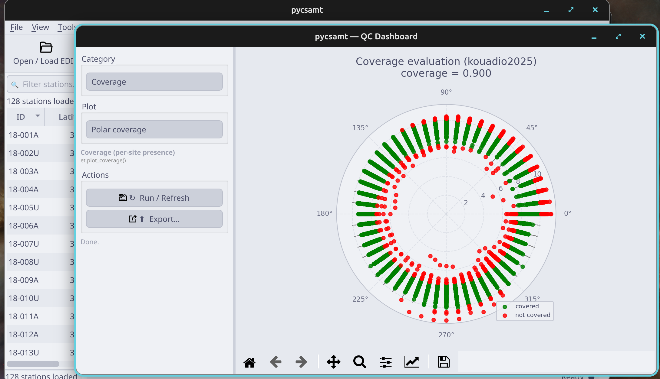
QC coverage dashboard for a loaded survey — Coverage diagnostics show whether stations and frequency bands are present enough to support downstream corrections and inversion preparation.#

Read this figure from left to right. First identify whether station coverage is continuous along the profile; abrupt vertical gaps usually point to missing or rejected bands at one station. Then inspect the frequency or period axis; horizontal gaps mean a band is missing across many stations and will affect any pseudosection or inversion mesh that expects continuous sampling. Finally, look for isolated weak stations. Those are candidates for station-level review in the profile viewer before any line-wide correction is attempted.

Use the coverage figure to decide:

whether the loaded files represent one coherent line;
whether all expected stations are present;
whether the usable frequency range should be narrowed;
whether a station should be flagged before inversion preparation;
whether a later contour, pseudosection, or depth slice is visually credible.

Do not use this figure to decide static shift by itself. Coverage tells you whether data exist; it does not tell you whether apparent resistivity is shifted by near-surface structure.

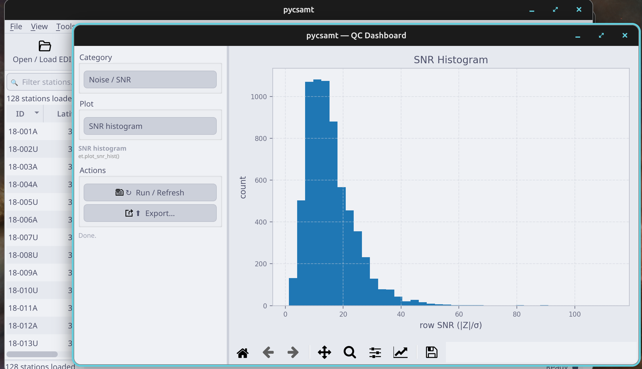
QC SNR diagnostic plot in the desktop dashboard — Noise and SNR diagnostics help decide whether to drop, mask, or smooth frequency bands before interpreting geoelectric structure.#

Read the SNR figure as a stability diagnostic. A line-wide low-SNR band can justify frequency editing or denoising. A single station with poor SNR should first be checked in the profile viewer, because the issue may be a bad station, missing component, local cultural noise, or import problem. Good SNR at short periods but poor SNR at long periods often means the deep part of the model will be weakly constrained.

Use the SNR figure to decide:

which frequency bands can be trusted in later phase-tensor and strike plots;
whether the noise-removal step should be station-specific or line-wide;
whether smoothing would hide a local problem rather than fix it;
whether inversion target bands should be reduced before input files are generated.

After any frequency edit or noise removal, return to this QC view. The goal is not to make the figure look clean at any cost; the goal is to remove bands that would otherwise dominate later interpretation with poor-quality evidence.

Practical QC checks:

Use coverage plots to find missing stations, missing bands, and line breaks.
Use SNR diagnostics before noise removal; do not smooth a whole line because one station has a local issue.
Use skew and dimensionality plots before assuming a 1-D, 2-D, or 3-D model.
Use static-shift and source-effect diagnostics to decide whether correction is justified.
Export figures that justify processing choices, especially for reports.

Data Corrections#

Open Data Corrections when QC shows a specific problem that should be handled before interpretation or inversion. The correction window is non-destructive: raw data stay available, previews are temporary, and applied steps live in a correction stack until they are committed.

The main correction families are static shift, noise removal, source effects, tensor rotation, coordinates, and Stratagem workflows. For impedance data, use Preview first, then Apply to add the result to the stack. Use Before / After, Overlay, Diff, and 2D Section views to compare the effect before committing.

Corrections are intentionally staged. Preview lets you see the result without changing the stack. Apply records one correction step in the local stack. Commit to Main is the state change that replaces the active survey for the rest of the desktop. Keep those three stages separate in your mind.

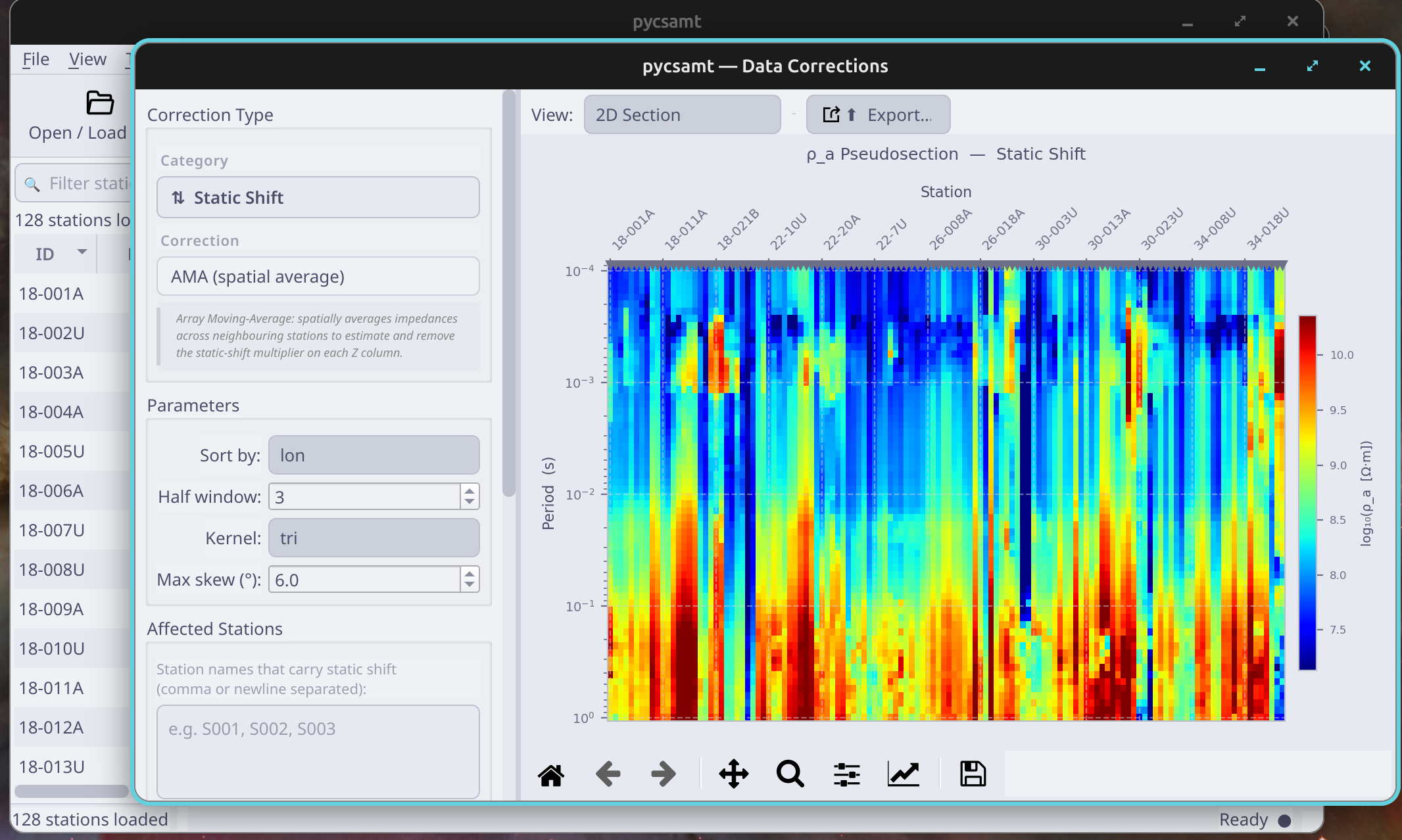
Static-shift correction panel with before and after plots — Static-shift correction should be reviewed station by station and on a pseudosection before it is committed to the active survey.#

This figure shows the correction window in its most important mode: a selected correction family on the left, parameters and affected stations below it, and before/after visual evidence on the right. Static shift changes apparent resistivity level without changing phase in the same way a true structural change would. That means the correction can be physically helpful when it is well justified, but dangerous when it is used only to make curves line up.

Read the static-shift figure in four passes:

Check the selected correction method and parameters. For AMA-style methods, the station half-window controls how local or smooth the correction is.
Compare the Before and After / Preview panels. Corrected curves should reduce station-to-station offsets without erasing real lateral geological contrasts.
Switch to Overlay or Diff when the change is subtle. Overlay shows shape preservation; Diff shows whether a correction is concentrated where you expected.
Use 2D Section for static shift because pseudosections reveal whether the corrected profile is more coherent along the line.

Commit this correction only when the factor is finite, positive, and supported by QC/static-shift diagnostics. If a strongly 3-D area causes the method to decline or return no useful factors, treat that as information rather than a failure to force through.

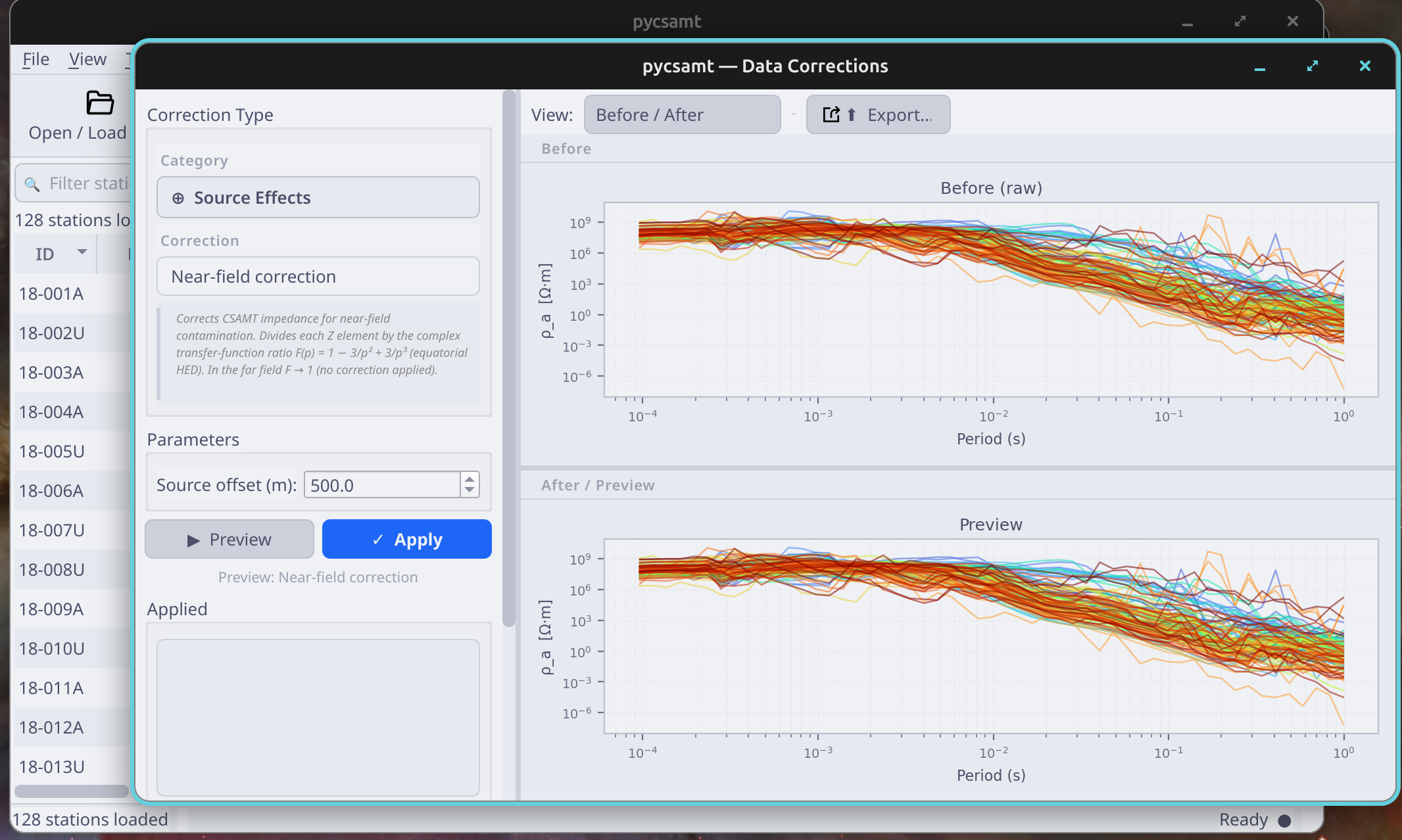
Source-effect correction view in the desktop correction window — Source-effect diagnostics are useful when response shape changes are tied to acquisition geometry or transmitter coupling rather than geology.#

This figure belongs later in the correction logic than static shift. Source effects can bias CSAMT responses when transmitter geometry, near-field behaviour, or acquisition coupling contaminates the response. The important visual clue is not simply that curves move; it is whether the movement follows a physically explainable source-effect pattern rather than arbitrary smoothing.

Use this figure to check:

whether the selected source-offset or source-effect parameters match the survey acquisition notes;
whether the strongest change occurs where the source-effect diagnostic predicted it;
whether phase and apparent-resistivity behaviour remain physically consistent after correction;
whether the correction should be exported as a separate product rather than silently replacing the normal corrected EDIs.

If the acquisition geometry is uncertain, save a figure and keep the output folder name explicit, for example corrected_source_effect_test. That makes it clear later that the output is conditional on a source-effect assumption.

Use Commit to Main only after the corrected curves and sections are credible. Committing sends the corrected Sites object back to the main desktop session, so the map viewer, profile viewer, QC dashboard, forward modelling, and inversion windows will work from the corrected data.

After committing any correction, immediately re-open the profile and QC views. The check is simple: the intended artifact should be reduced, and no new station-order, component, or response-shape problem should appear.

Advanced Diagnostics#

Open Advanced Tools when QC indicates that the survey needs deeper interpretation before correction or inversion. This window collects analyses that are useful but too specialized for the first-pass dashboard: strike analysis, dimensionality views, topography preview, sensitivity checks, and format conversion tools.

Advanced diagnostics are used to defend assumptions. They should answer questions such as: “Can I rotate to a single regional strike?”, “Is a 2-D profile assumption reasonable?”, “Does topography need to be carried into the model?”, and “Is this converted data set spatially coherent?”

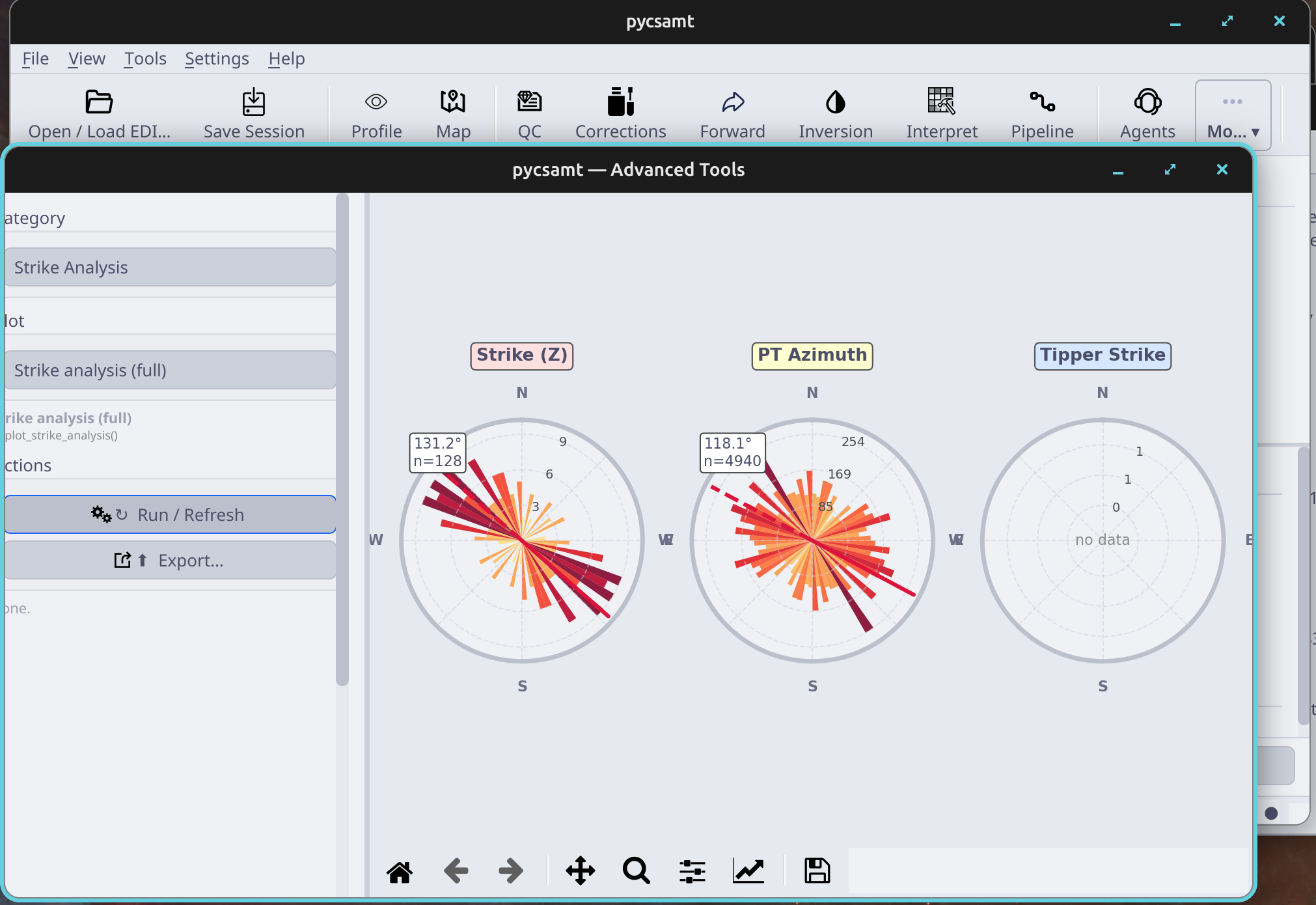
Full strike analysis panel in Advanced Tools — Strike analysis compares direction estimates across stations and periods so a rotation angle is not chosen from a single noisy diagnostic.#

The full strike-analysis figure is the high-level strike summary. It brings together rose-style direction statistics and stability information so you can see whether a dominant direction is persistent or only appears in one station or period band. A strong strike decision should appear as a stable cluster, not as a scattered set of unrelated azimuths.

Use this figure before tensor rotation or 2-D inversion setup. If the strike direction is stable over the period band that matters for the target depth, then a rotation step can be justified. If the strike is unstable, multi-modal, or changes strongly along the profile, document that uncertainty and avoid pretending that one angle is a survey-wide truth.

Questions to ask while reading it:

Is there one dominant azimuth or several competing directions?
Does the preferred direction persist across the useful period band?
Are outlier stations controlling the summary?
Does the strike agree with map-view line direction and known geology?

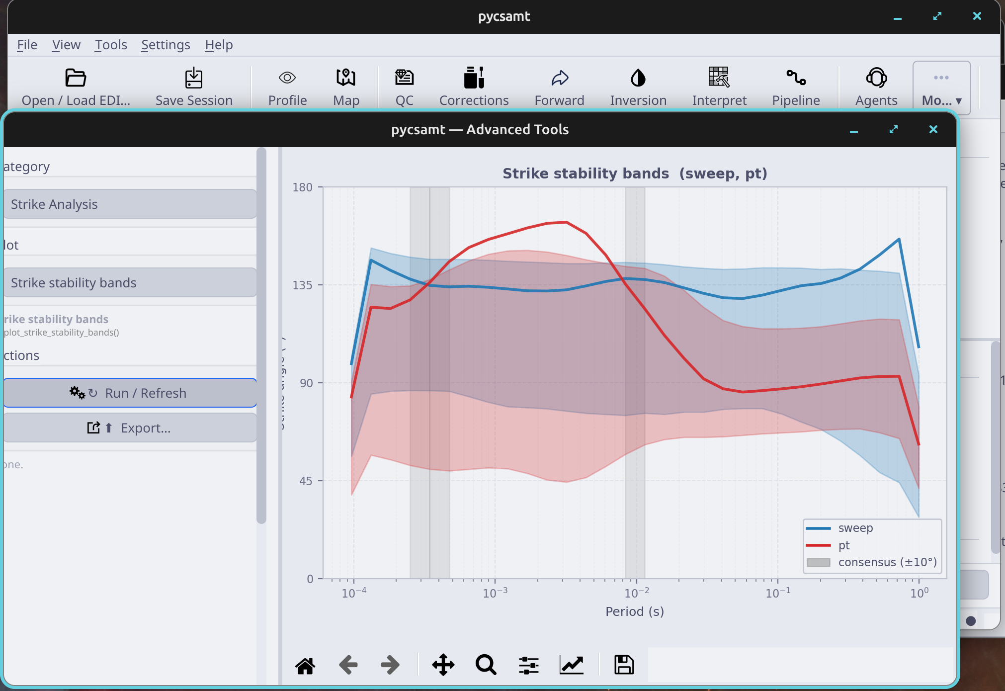
Strike stability bands in Advanced Tools — Stability bands highlight whether a strike estimate is persistent across the frequency or period range used for interpretation.#

The stability-band figure is more diagnostic than decorative. It shows where strike estimates are stable enough to trust and where they become ambiguous. Stable bands support choosing a rotation angle for a selected period range. Unstable bands warn you that the data may be 3-D, noisy, or affected by local near-surface structure.

Use this figure to choose the period interval that feeds the rotation or inversion assumption. Do not average all periods blindly. A shallow stable band may support near-surface interpretation, while a deeper band may need a different assumption or no rotation at all.

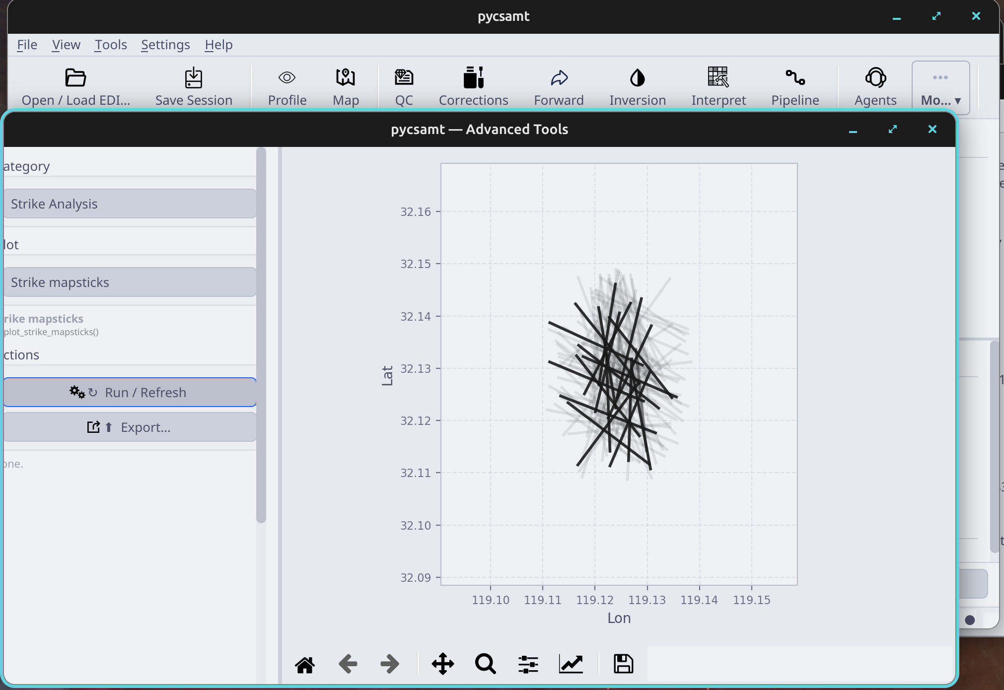
Strike mapsticks plotted along station locations — Mapsticks make it easier to see whether station-level strike directions change with location along the survey line.#

Mapsticks translate strike estimates into spatial context. Each station-level stick should be read against the station geometry and profile direction. A smooth spatial trend may indicate changing geology; a single station with a very different stick may indicate a local data issue or distortion.

Use this figure when the rose summary looks plausible but you need to know whether the direction is line-wide. If the mapsticks rotate progressively along the line, consider segmenting the interpretation or documenting a spatially varying strike. If they are random, do not use a single rotation angle without further QC.

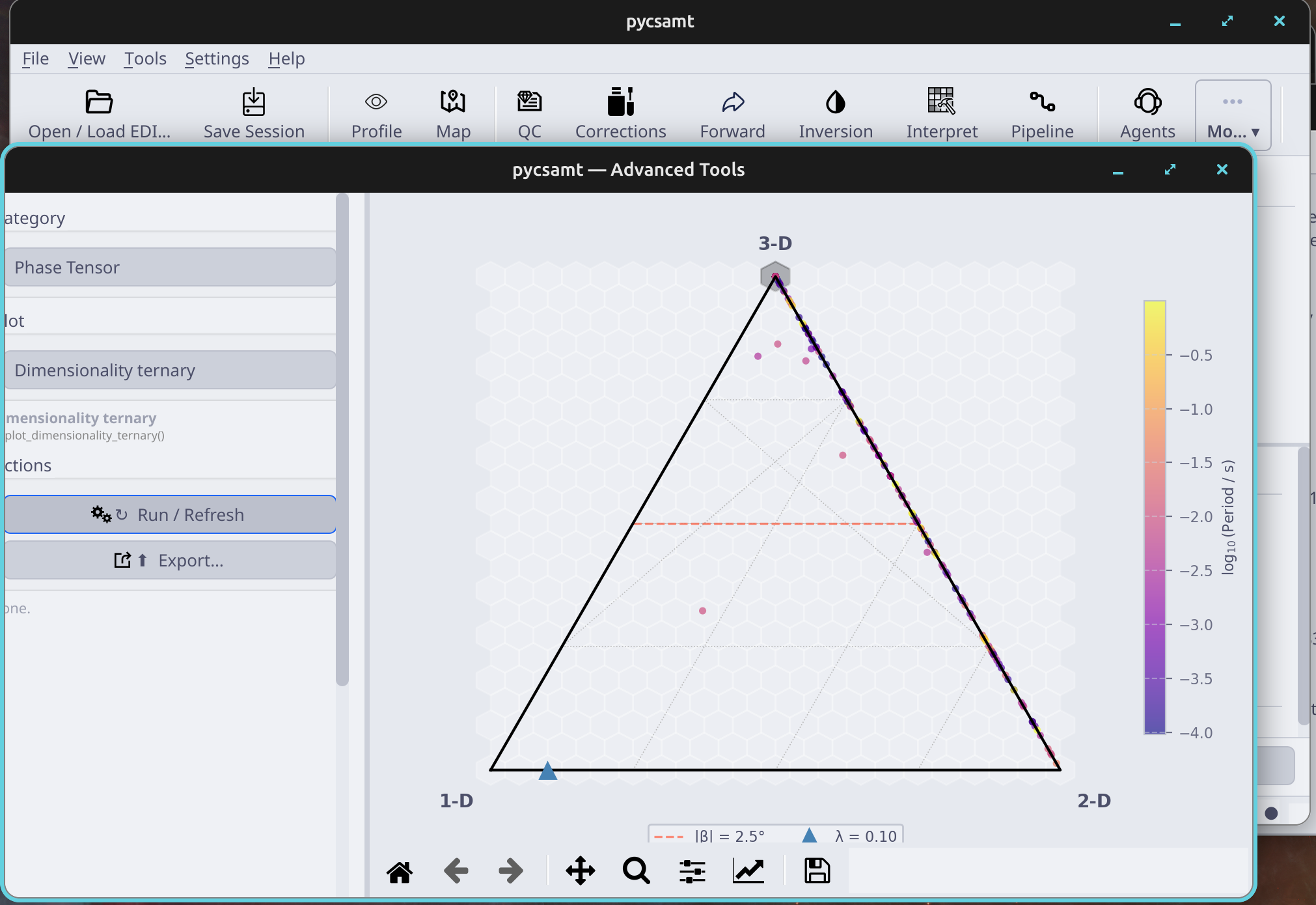
Dimensionality ternary diagnostic in the desktop tools — Dimensionality diagnostics help decide whether a 1-D assumption is still defensible, or whether 2-D/3-D interpretation should be used.#

The ternary dimensionality figure summarizes whether stations and period bands behave more like 1-D, 2-D, or 3-D responses. Treat it as an assumption check before modelling. A strong 1-D cluster supports 1-D forward tests and simple layered inversions. A strong 2-D signal supports profile interpretation with strike care. A broad or 3-D-heavy spread means the inversion and correction strategy should be more cautious.

This figure is especially important when a smooth profile plot tempts you into a simple model. Smooth apparent-resistivity curves do not prove 1-D geology; phase tensor and dimensionality diagnostics provide the stronger evidence.

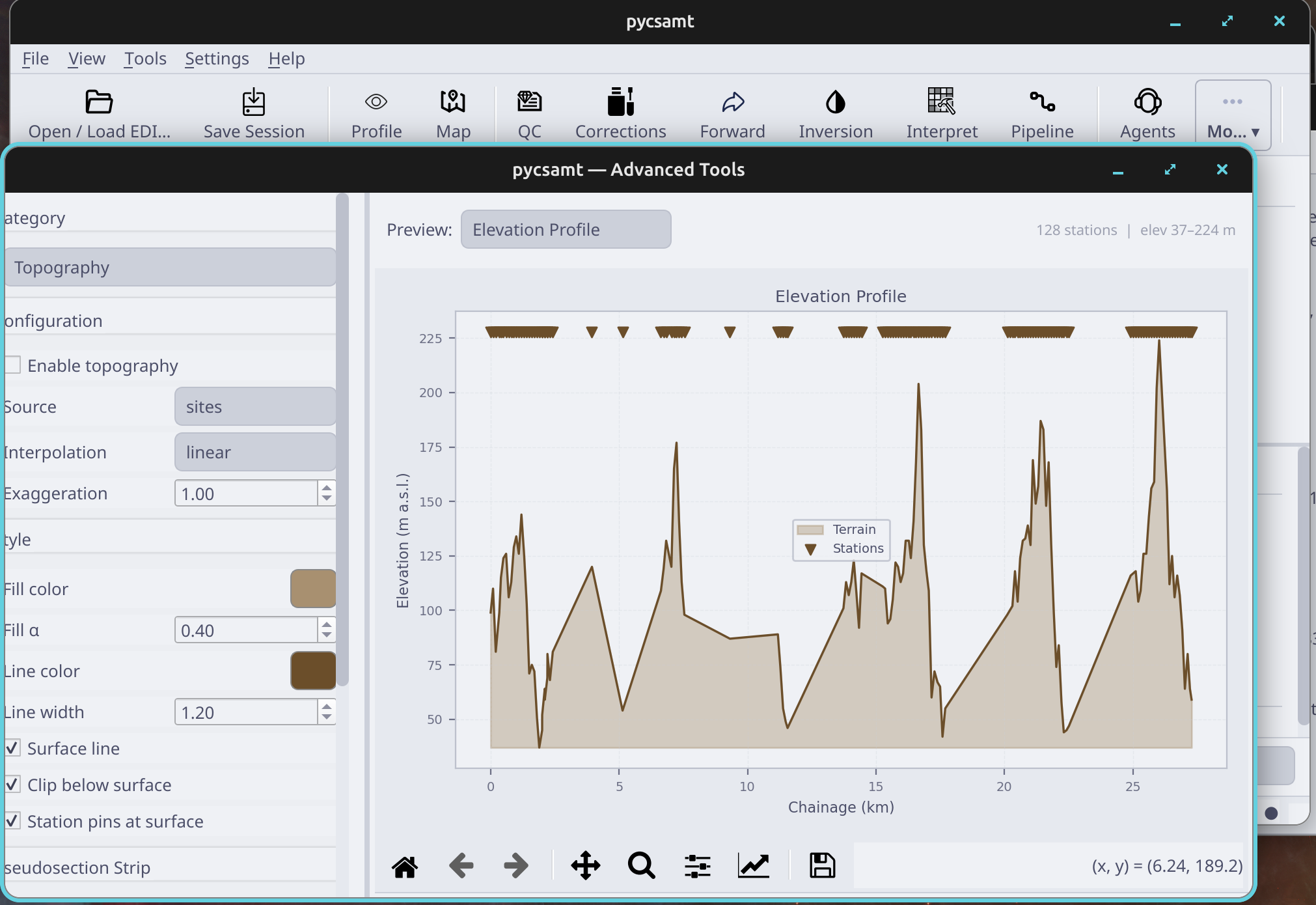
Topography preview in Advanced Tools — Topography preview checks elevation and station-position information before those values are written into converted or corrected products.#

The topography figure checks whether elevation and profile geometry are safe to carry into conversion, forward modelling, or inversion input files. Look for missing elevations, unrealistic spikes, reversed station order, and coordinate jumps. These issues can make a physically reasonable model appear wrong because the survey geometry is wrong.

Use topography preview before exporting converted EDIs or building inversion inputs. If elevation has been corrected or imported from an external source, save the preview figure with the converted output so the geometry decision is traceable.

Advanced Tools can also convert AVG, J, and Spectra files to EDI. When using conversion, preview the station profile and topography first, write EDIs to a dedicated output folder, then reload the exported EDIs as a normal survey.

Forward Modelling#

Open Forward Modelling when you need synthetic responses, a conceptual starting model, or a controlled comparison before inversion. The window has a model builder, result tabs, and a small library/preset panel. It supports 1-D, 2-D, and 3-D forward configurations, with 1-D model saving and geological presets for quick starts.

Forward modelling is not the inversion result. It is a controlled experiment: change the model, compute the response, and learn which features of the data could plausibly come from which resistivity structures.

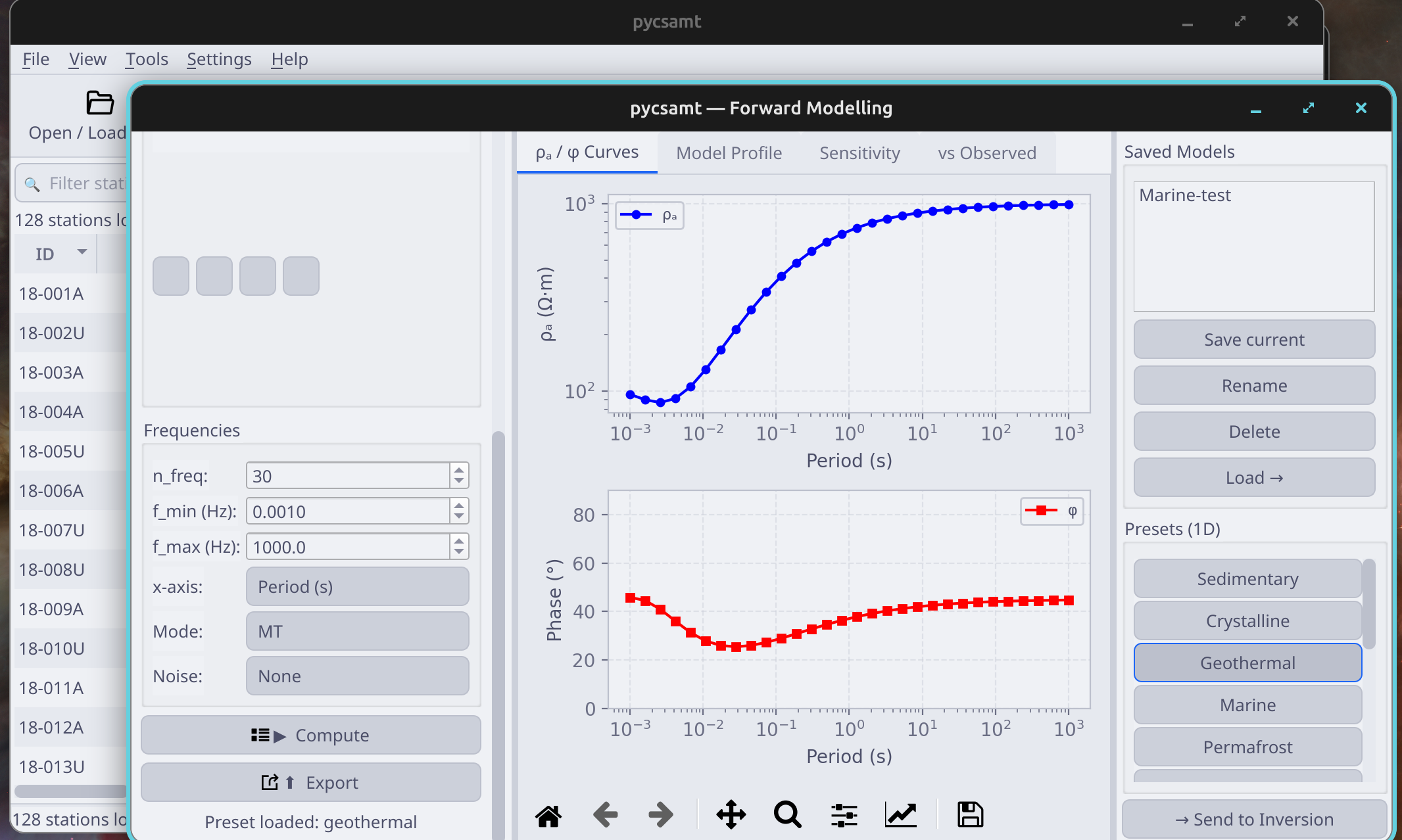
Geothermal preset loaded in the forward modelling window — Geological presets provide quick initial models that can be edited before computing synthetic responses.#

This figure shows the model-builder side of the workflow. A preset loads a geologically plausible starting resistivity structure, but it is only a prior. Edit the layer values, thicknesses, grid size, anomaly parameters, and frequency sampling so the forward model matches the question you are asking.

Use presets for:

a fast first model when the target setting is known;
teaching the inversion window a reasonable starting structure;
comparing how different geological scenarios change the response;
creating a reproducible baseline before manual model edits.

Do not treat a preset name as interpretation proof. The synthetic response must still be compared with observed station profiles and QC constraints.

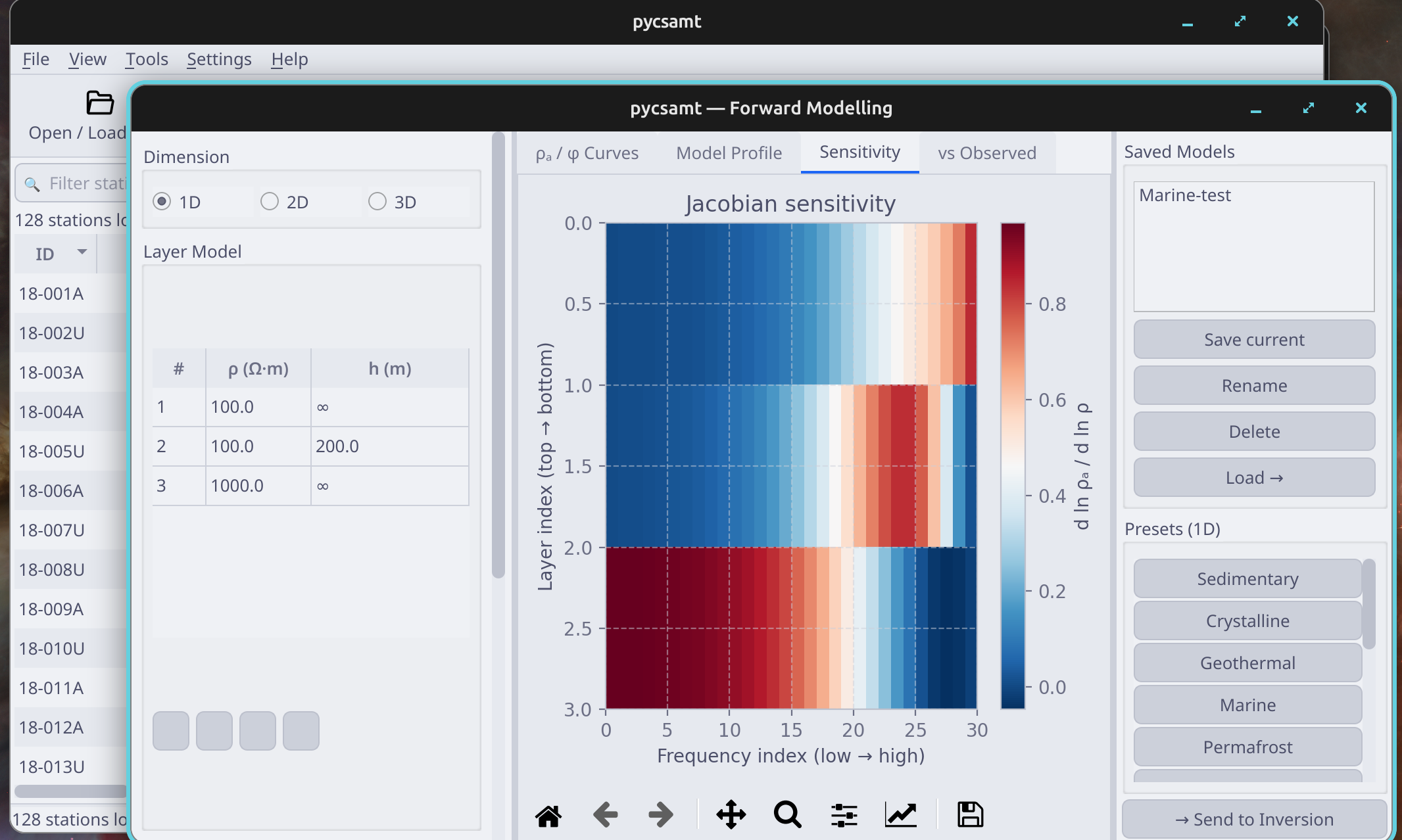
1-D sensitivity plot in the forward modelling window — Sensitivity views show which layers and frequencies control the response.#

The 1-D sensitivity figure answers a practical question: which layers are actually constrained by the selected frequency band? Strong sensitivity means the response changes when that layer changes. Weak sensitivity means inversion may fit the data while leaving that part of the model poorly resolved.

Use this figure before trusting deep layers. If the frequency coverage has little sensitivity to the depth interval of interest, the inversion may still produce a model, but the deep structure should be reported with caution. This is also where QC and forward modelling meet: if SNR removed long periods, the deep sensitivity may be reduced.

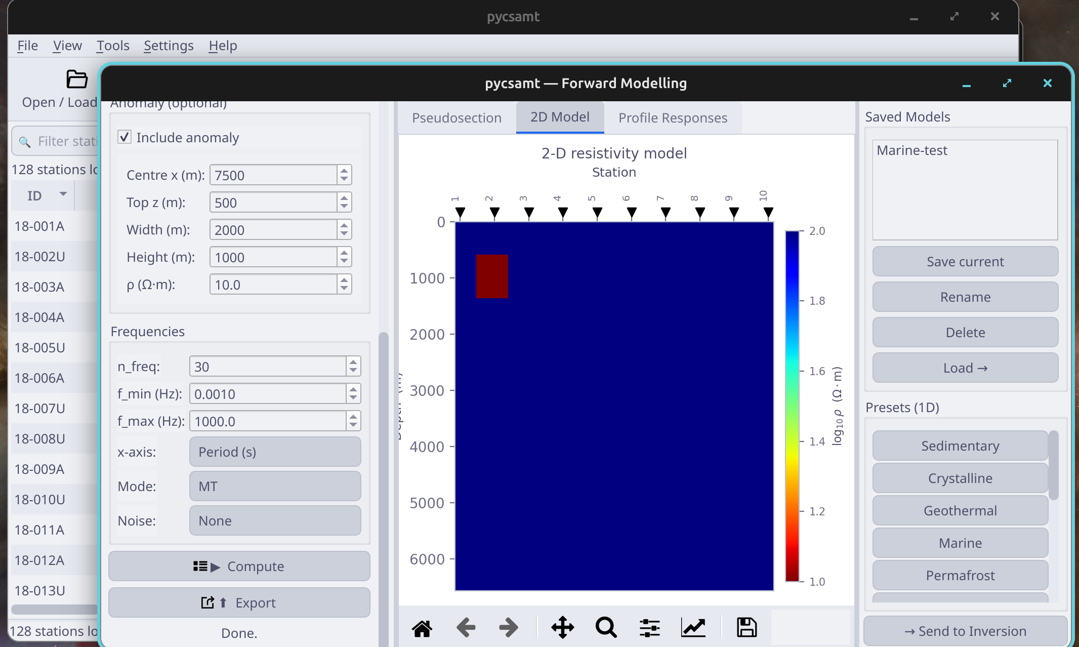
2-D resistivity model in the forward modelling window — A 2-D model view makes the geometry of background resistivity and anomalies explicit before response plots are interpreted.#

The 2-D model figure is the physical hypothesis. Read the axes, background resistivity, anomaly geometry, and station placement before looking at the response. A synthetic response is meaningful only if the model geometry is geologically plausible and sampled by stations in a way that resembles the real survey.

Use this figure to check:

whether the anomaly is inside the station aperture;
whether padding and grid spacing are large enough for stable responses;
whether the model depth range covers the period band being interpreted;
whether topography or station spacing should be represented more carefully.

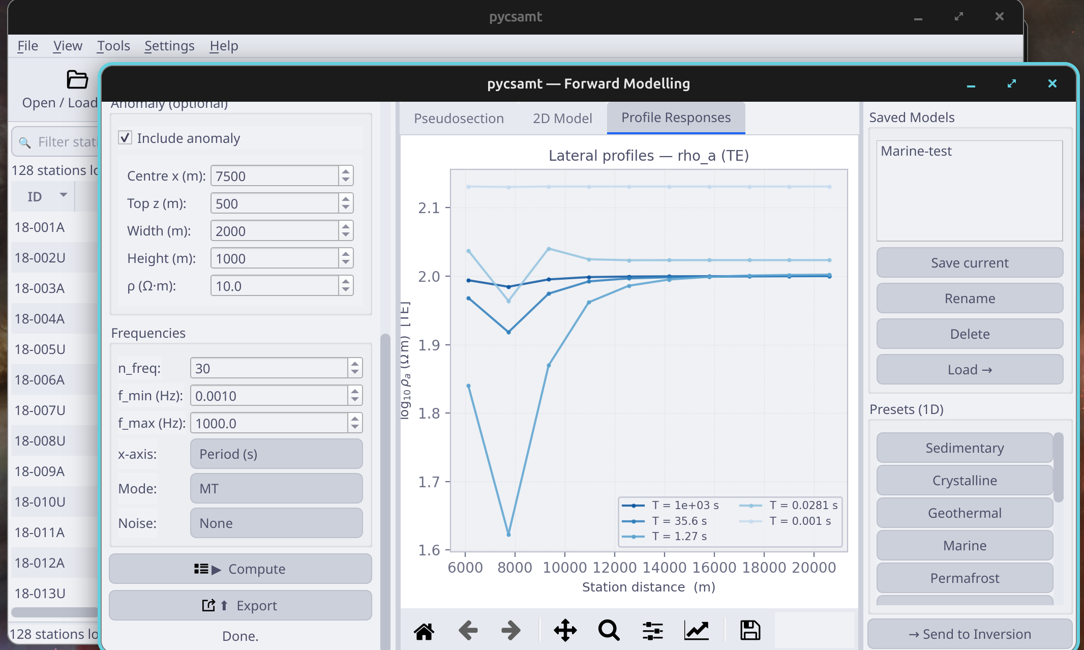
Profile responses are useful for comparing synthetic station behaviour with the observed profile viewer.#

The 2-D profile-response figure is the bridge between hypothesis and data. It shows how the model would appear as station responses along the profile. Compare broad patterns rather than forcing exact agreement: where does the response rise or fall, where are gradients strongest, and which stations carry the anomaly signature?

Use this figure before sending a model to inversion. A good starting model does not need to fit perfectly, but it should put resistive and conductive features in reasonable places and should not contradict the strongest observed profile trends.

Use Send to Inversion when the forward model should seed the inversion panel. The handoff carries the model parameters, and the inversion window can load them as the starting model.

Inversion Preparation#

Open Inversion Wizard after QC, correction, and strike decisions are stable. The desktop inversion panel includes traditional engines such as Occam2D, ModEM, and MARE2DEM, plus AI inversion modes for supported dimensions. External solver binaries are optional paths; pyCSAMT can still build input files in the selected working directory.

The inversion window is where earlier uncertainty becomes configuration. A poor QC decision becomes a bad frequency band. An uncertain strike decision becomes a questionable rotation. An undocumented static-shift correction becomes an output that cannot be audited. Use the window only after those choices are visible in saved figures or notes.

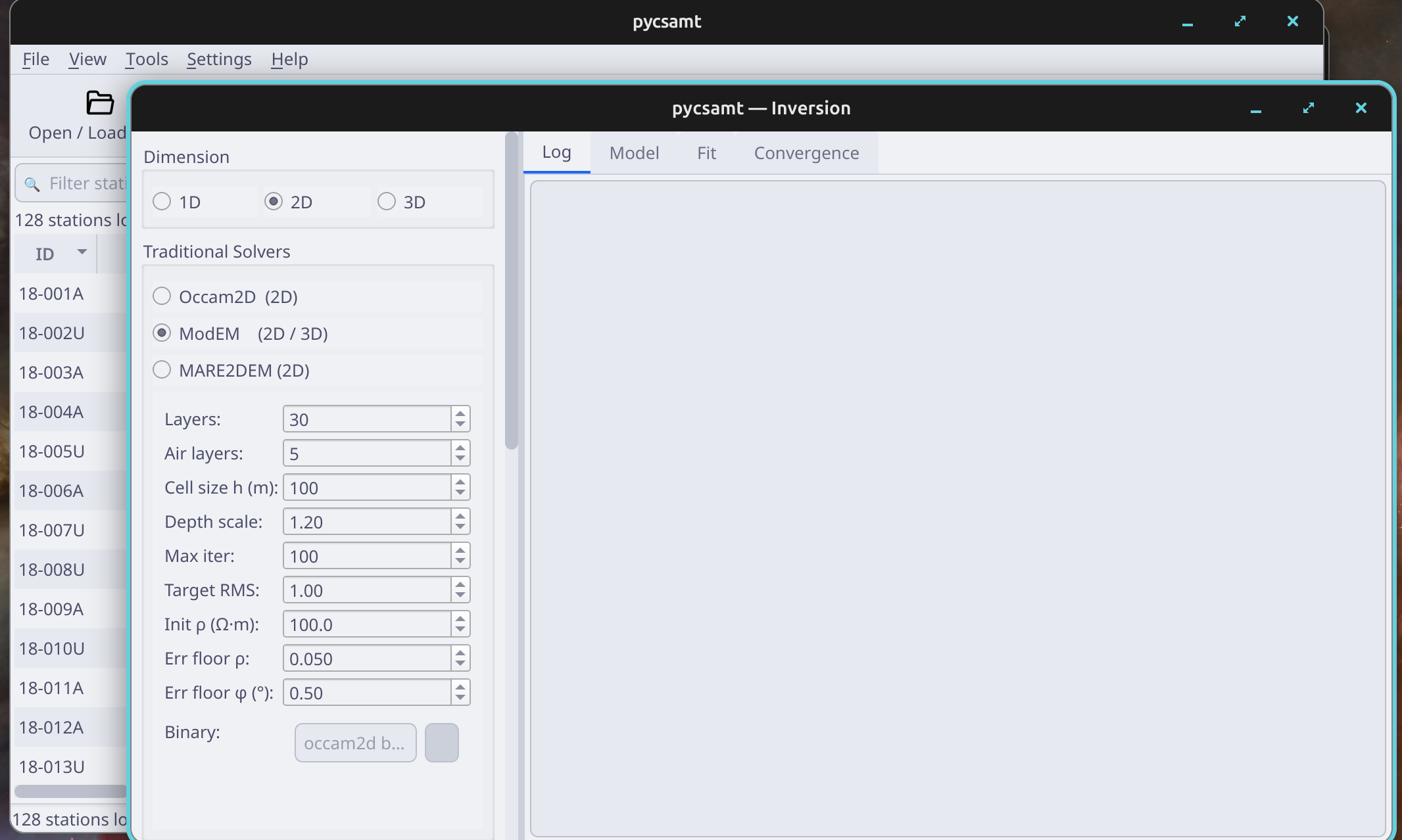
Desktop inversion wizard home view — The inversion window collects engine choice, dimensionality, starting model, data options, output directory, and run logs in one place.#

Read this figure as a checklist, not just a launch screen. The left side of the inversion panel controls the scientific setup: dimensionality, engine, starting model, and solver-specific parameters. The working directory and log area define the reproducibility boundary: every generated input file, solver log, and result should belong to one named run folder.

Use the inversion figure to verify:

Engine – Occam2D, ModEM, MARE2DEM, or AI inversion matches the data assumption and available solver environment.
Dimension – the selected dimension is supported by QC, strike, and dimensionality diagnostics.
Starting model – the model is imported from Forward Modelling or built intentionally, not accepted by accident.
Workdir – the folder name identifies survey line, data state, engine, and run attempt.
Logs – input-building messages are read before a long solver run starts.

For traditional external solvers, building input files successfully is a useful milestone even if the binary is not run immediately. Review those files before committing compute time to an inversion.

Before pressing Run, check:

the active survey is the intended raw or corrected data set;
the working directory is specific to this run;
the dimensionality matches QC and strike diagnostics;
the starting model is documented or imported from Forward Modelling;
external binary paths are set for solver runs that need them;
generated input files are reviewed before long external inversions.

Processing Pipeline#

Use Processing Pipeline after the manual workflow is understood. The pipeline is for repeatability: it applies a known sequence with saved parameters, logs each step, previews diagnostics, and can export the final EDI collection.

The pipeline is not the place to discover the right processing choices for the first time. Use the manual panels to learn what a survey needs; then encode those choices into the pipeline so the same line, or a similar line, can be processed consistently.

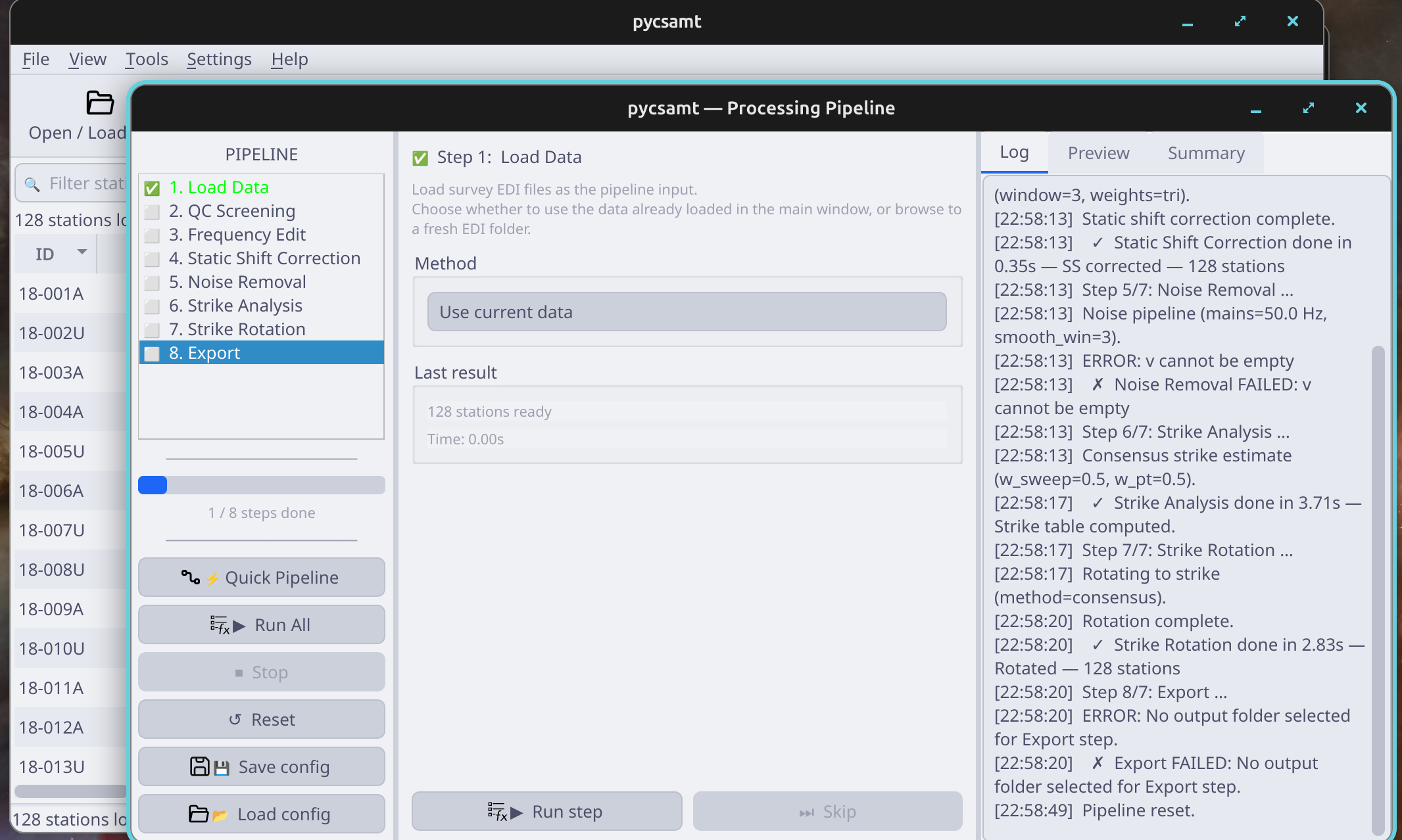
Desktop processing pipeline stepper and preview window — The pipeline window uses a stepper on the left, method and parameter controls in the centre, and log/preview/summary tabs on the right.#

This figure has three functional regions. The left stepper tells you where the run is in the eight-step chain and whether each step is pending, running, done, skipped, or errored. The centre panel is the contract for the selected step: method choice plus parameters. The right tabs are the evidence trail: the log records what happened, the preview shows a diagnostic for the selected step, and the summary captures the final status.

Read the pipeline figure before pressing Run All:

If step 1 is Use current data, confirm the main window is showing the intended raw or corrected survey.
If a step is skipped, write down why it is skipped. A skipped rotation is a scientific decision when strike is unstable.
If a step has parameters, compare them with the manual correction or QC settings that were already tested.
If a preview plot looks worse than the manual result, stop and run that step alone with adjusted parameters.
If export is the final step, choose a new output folder for that pipeline attempt.

The pipeline gives you repeatability, but it also multiplies mistakes quickly. Run one step at a time while tuning, then use Run All only when the chain has already produced acceptable intermediate diagnostics.

The built-in sequence is:

Load Data – use the current survey or browse to an EDI folder.
QC Screening – flag or drop low-confidence frequencies.
Frequency Edit – edit, close gaps, or regrid frequency bands.
Static Shift Correction – apply AMA, LOESS, bilateral, or reference median correction.
Noise Removal – run automatic filtering, EMAP, or robust PCA denoising.
Strike Analysis – estimate regional strike by consensus, phase tensor, or sweep methods.
Strike Rotation – rotate tensors to strike or intentionally skip.
Export – write processed EDI files to the chosen output folder.

Run a single step when tuning parameters. Use Quick Pipeline only after the default choices are acceptable for that survey family. Save the pipeline configuration beside the exported EDIs so the processing can be reproduced.

Suggested pipeline naming:

pipeline/
  L30_raw_to_qc_ss_rotate_2026-07-02.json
  L30_raw_to_qc_ss_rotate_2026-07-02.log
  exported_edi/

The name should describe the input state and the main processing choices. A generic name such as run1 is hard to audit later.

Agent-Assisted Review#

The desktop agent panels can help explain QC or inversion results after the scientific checks are visible. Use them as a review layer, not as a replacement for diagnostic plots.

Agent review is most useful after figures exist. Ask the agent to summarize patterns, compare diagnostics, or explain why a workflow step might be risky. Do not ask it to decide corrections without the QC and profile evidence open.

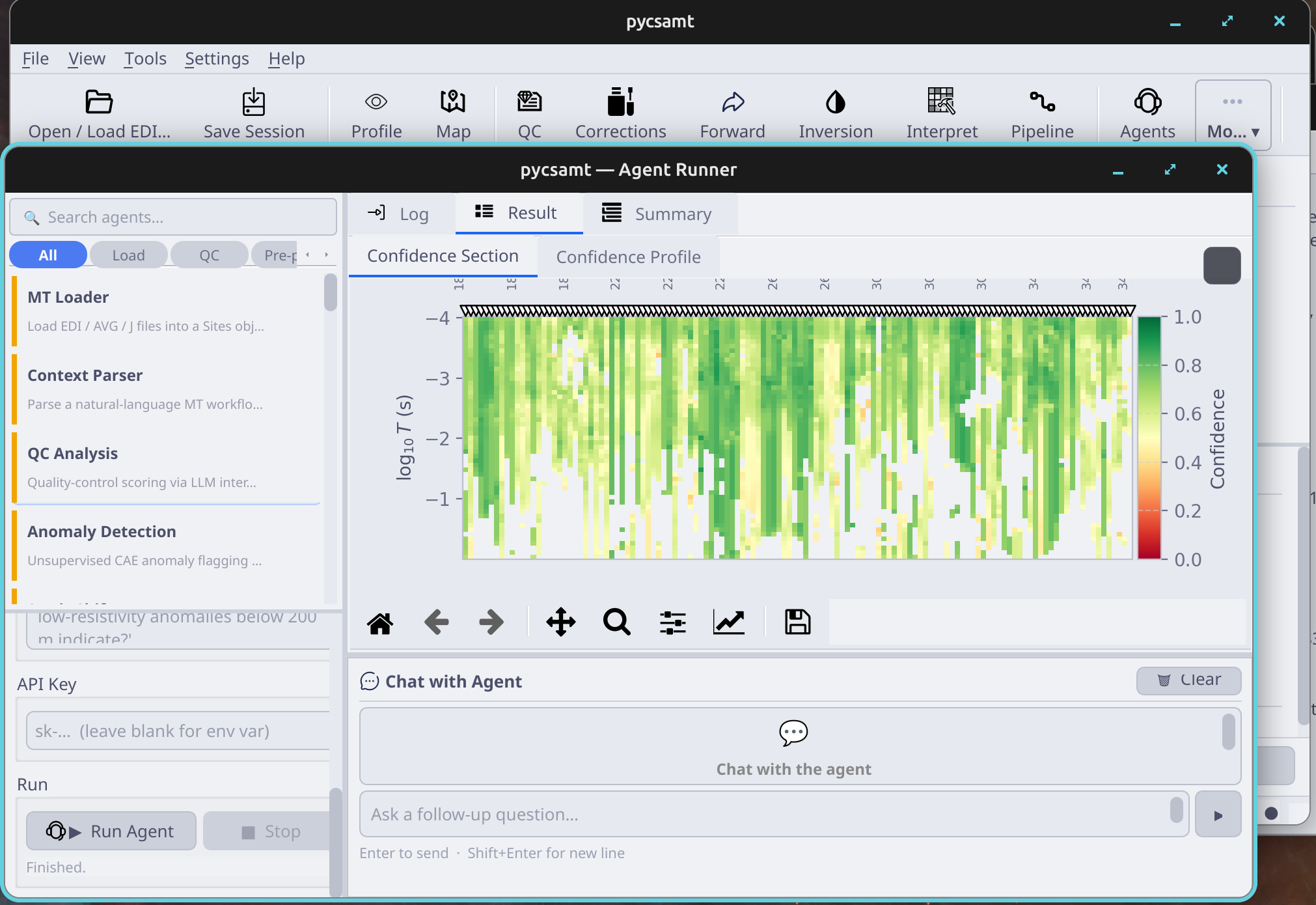
Agent confidence summary for desktop processing — Confidence summaries are useful for documenting which stations or bands need closer review.#

The confidence figure is a triage view. It helps identify which stations, frequency bands, or workflow areas deserve human attention. High confidence does not prove a model is correct; it means the available checks agree more strongly. Low confidence should trigger a return to QC, profile, map, or correction views.

Use this figure to write review notes:

which stations need inspection;
which bands were weak or removed;
which correction assumptions were strong or uncertain;
which later inversion decisions should be treated cautiously.

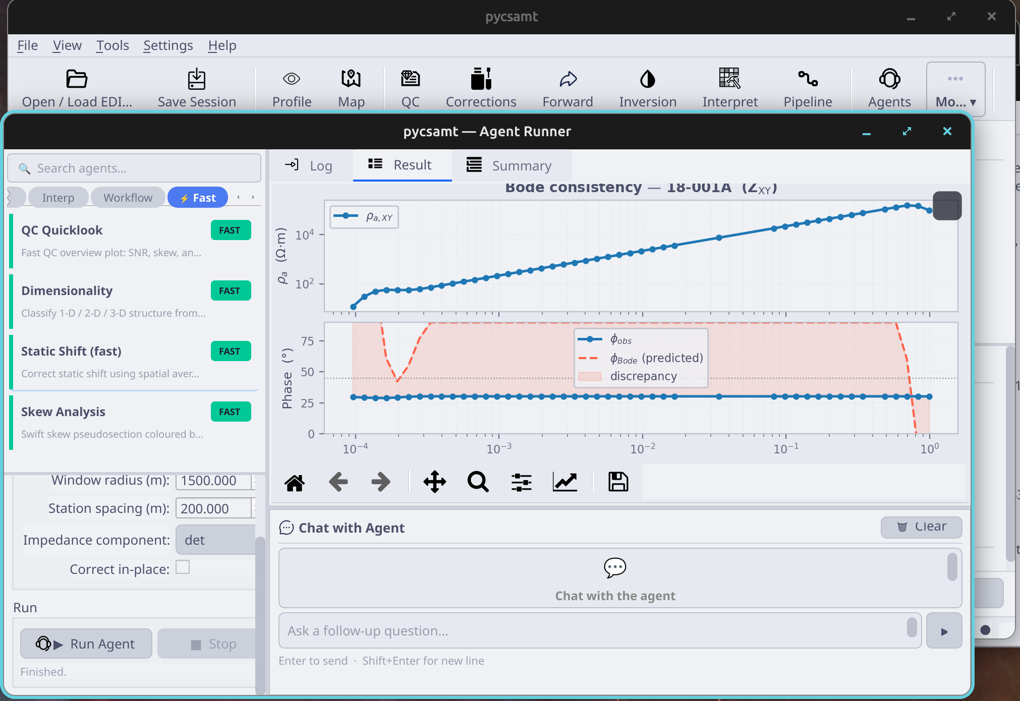
Agent Bode consistency diagnostic in the desktop application — Consistency checks should be compared with the profile and QC windows before changing data or inversion settings.#

The Bode-consistency figure checks whether apparent resistivity and phase behaviour are mutually plausible. It is a useful warning system for component issues, noisy bands, or responses that need station-level review. Treat it as an explanation aid: when it flags a station, go back to the profile viewer and look at the underlying curves.

Do not apply a correction only because an agent panel marks a concern. Use the concern to navigate to the relevant diagnostic, then make the processing decision from the data view.

Outputs And Reproducibility#

Keep each processing attempt in its own output folder. A practical layout is:

raw/ for untouched source EDI files;
qc/ for first-pass figures and tables;
corrected_edi/ for committed correction outputs;
pipeline/ for saved pipeline JSON, logs, and final EDIs;
forward/ for synthetic models and exported figures;
inversion/<run_name>/ for solver input files, logs, and results;
session/ for the saved desktop session file.

The important rule is simple: every exported data product should have the figures and parameters that explain how it was produced.

For each processing stage, save one evidence figure and one machine-readable configuration when available:

Stage	Save	Why It Matters
QC	Coverage, SNR, skew/dimensionality figures	Shows which data were trusted or rejected.
Corrections	Before/after or diff figures plus corrected EDIs	Proves what changed before the active survey was replaced.
Advanced diagnostics	Strike, dimensionality, and topography figures	Documents rotation, model dimension, and geometry assumptions.
Forward modelling	Model plots, responses, and starting-model parameters	Explains the prior used for inversion.
Inversion	Input files, run logs, result figures	Makes the solver run auditable and repeatable.
Pipeline	Pipeline JSON, log, preview/summary figures	Recreates the exact automated processing chain.

When a result is shared, the output folder should let another user reconstruct the chain without relying on memory or screenshots alone.