16.14. From Forward Modelling To Inversion#

Forward modelling and inversion are the two directions of the same forward operator. A forward model predicts observations from a known earth model:

(1)#\[d_{\mathrm{pred}} = F(m).\]

An inversion runs the same operator inside a search, adjusting \(m\) until predicted and observed data agree while the model itself stays well behaved:

(2)#\[\Phi(m) = \Phi_d(m) + \lambda \Phi_m(m), \qquad \Phi_d(m) = \left\| W_d \left(d_{\mathrm{obs}} - F(m)\right) \right\|_2^2.\]

\(W_d\) contains the data uncertainties, \(\Phi_m\) is the model penalty, and \(\lambda\) controls the trade-off between fitting the data and keeping the model simple – see Forward Modelling Concepts and Inversion Concepts for how each piece is built up.

In pyCSAMT, the forward package helps answer the question:

“If this geology existed, what would the survey measure?”

The inversion package helps answer the complementary question:

“Given what the survey measured, which class of models can explain it?”

The bridge between the two is not only a Python object. It is a modelling contract: units, shapes, station geometry, noise assumptions, model parameterization, and backend dimensionality must remain consistent.

16.14.1. The Handoff Contract#

Before sending synthetic or field data to an inversion backend, make the following contract explicit.

Item	Forward-side meaning	Inversion-side requirement
Method	MT, AMT, CSAMT, EMAP, or TDEM response type.	`InversionConfig.method` must match the data family.
Dimensionality	1-D layered model, 2-D profile, or quasi-3-D grid.	`InversionConfig.dimension` and `backend` must support the same interpretation.
Frequency or time axis	`freqs` for frequency-domain responses, `times` for TDEM gates.	Axis order must match every response array.
Response arrays	Apparent resistivity and phase, or TDEM decay values.	Use backend-neutral keys such as `rho_a`, `phase`, and `values`.
Station geometry	Station positions created by a profile or grid.	Preserve `station_x` and `station_names` for profile inversions.
Error model	Noise added to synthetic data, or field uncertainty estimates.	Configure `error_floor`, `phase_error`, or explicit errors.
Starting model	A plausible low-resolution model, not the hidden truth.	Provide `StartingModel` or a compatible mapping when the backend uses layered parameters.
Truth model	The known model used in a synthetic recovery experiment.	Store it as metadata or in the experiment archive for later comparison.

The most common backend-neutral data mappings are:

Workflow	Data keys	Array convention
MT, AMT, CSAMT 1-D	`freqs`, `rho_a`, `phase`	`rho_a` and `phase` are one-dimensional arrays with length `n_frequencies`.
TDEM 1-D	`times`, `values`	`values` is a one-dimensional decay array with length `n_times`.
Frequency-domain profile	`freqs`, `rho_a`, `phase`, `station_x`	`rho_a` and `phase` use shape `(n_stations, n_frequencies)`.
TDEM profile	`times`, `values`, `station_x`	`values` uses shape `(n_soundings, n_times)`.
Native external run	Backend-specific files and options.	Use the model backend page for native file generation and execution.

The forward 2-D response containers store frequency first, for example response.rho_a_te has shape (n_frequencies, n_stations). The inversion profile API expects station first. Transpose the arrays when moving directly from MT2DForward to a profile inversion.

16.14.2. Why Synthetic Recovery Comes First#

A forward response shows whether a target can influence the data. A synthetic recovery test checks whether the planned inversion can recover that influence under realistic assumptions. This is a different and stricter question.

A useful recovery loop is:

define a known truth model;
compute the clean forward response;
add controlled noise;
choose an inversion parameterization and starting model;
invert the synthetic data;
compare recovered and true models;
inspect residuals, uncertainty, convergence history, and artefacts;
repeat with modified frequency range, station spacing, noise, and regularization.

The test should include at least one easy model and one difficult model. The easy model confirms that the mechanics are correct. The difficult model exposes non-uniqueness, poor sensitivity, and resolution limits.

16.14.3. 1-D MT Recovery#

The smallest complete bridge is a 1-D layered MT recovery. The forward response is converted into the backend-neutral inversion mapping using freqs, rho_a, and phase. Paste the whole block into a script: it builds the truth model, the noisy synthetic data, and the inversion configuration in one pass.

>>> import numpy as np

>>> from pycsamt.forward import FieldRealisticNoise, LayeredModel, MT1DForward
>>> from pycsamt.inversion import InversionConfig, InversionWorkflow, StartingModel

>>> freqs = np.logspace(-2, 2, 16)

>>> truth = LayeredModel(
...     resistivity=[80.0, 25.0, 600.0],
...     thickness=[250.0, 900.0],
... )

>>> clean = MT1DForward(freqs=freqs).run(truth)
>>> noisy = FieldRealisticNoise(base_level=0.05).apply(clean, seed=42)

>>> cfg = InversionConfig(
...     method="mt",
...     dimension="1d",
...     backend="builtin",
...     data={
...         "freqs": freqs,
...         "rho_a": noisy.rho_a,
...         "phase": noisy.phase,
...     },
...     starting_model=StartingModel(
...         resistivities=[100.0, 50.0, 500.0],
...         thicknesses=[300.0, 1000.0],
...     ),
...     error_floor=0.05,
...     phase_error=3.0,
...     regularization="smooth",
...     max_iter=25,
...     metadata={
...         "experiment": "synthetic_mt_1d_recovery",
...         "noise_seed": 42,
...     },
... )

>>> result = InversionWorkflow(cfg).run()

>>> print(result.summary())
InversionResult(method='mt', dimension='1d', backend='builtin', status='converged', rms=0.851)
>>> recovered = result.model
>>> print("recovered resistivities:", np.round(recovered.resistivities, 1))
recovered resistivities: [ 74.3  25.6 596. ]
>>> print("truth resistivities:    ", truth.resistivity)
truth resistivities:     [ 80.  25. 600.]

The starting model was off by 20-100% on every layer, and 25 iterations were enough to land within a few percent of the truth on all three – the middle conductive layer, which dominates the mid-period response, recovers almost exactly. Plotting the two side by side makes the same point visually:

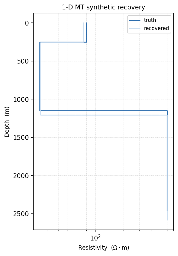
Recovered 1-D MT resistivity model overlaid on the true model — Truth and recovered models, plotted with `pycsamt.forward.plot.plot_model_1d()`.#

Use the result diagnostics, not only the recovered layer values, to judge whether that agreement is trustworthy rather than lucky:

>>> if result.history is not None:
...     history = result.history.arrays()
...     print("objective (final):", round(float(history["objective"][-1]), 4))
...     print("rms (final):", round(float(history["rms"][-1]), 4))
...
objective (final): 23.1926
rms (final): 0.8513
>>> if result.uncertainty is not None:
...     print("uncertainty.confidence shape:", result.uncertainty.confidence.shape)
...
uncertainty.confidence shape: (3, 1)

>>> model_for_export = result.to_resistivity_model()
>>> print("model_for_export.method:", model_for_export.method)
model_for_export.method: builtin:mt:1d

An RMS misfit near 1 means the recovered model fits the noisy data about as well as the assigned 5% error floor and 3-degree phase error allow – neither over-fitting the noise nor leaving obvious structure unexplained.

Important interpretation points:

truth is used only to generate the data and to evaluate recovery.
starting_model is the model supplied to the inversion. It should be plausible, but it should not secretly duplicate the truth.
error_floor should be compatible with the noise injected into noisy. A smaller error floor asks the inversion to fit data more tightly.
phase_error is in degrees and controls the phase contribution when phase observations are included.

16.14.4. 1-D TDEM Recovery#

TDEM uses a time axis and decay values rather than apparent resistivity and phase. The backend-neutral mapping therefore uses times and values.

>>> import numpy as np

>>> from pycsamt.forward import LayeredModel, TEM1DForward
>>> from pycsamt.inversion import InversionConfig, InversionWorkflow, StartingModel

>>> times = np.logspace(-5, -3, 8)

>>> truth = LayeredModel(
...     resistivity=[60.0, 250.0, 900.0],
...     thickness=[120.0, 700.0],
... )

>>> forward_options = {
...     "loop_radius": 25.0,
... }

>>> clean = TEM1DForward(times=times, **forward_options).run(truth)

>>> cfg = InversionConfig(
...     method="tdem",
...     dimension="1d",
...     backend="builtin",
...     data={
...         "times": times,
...         "values": clean.dBz_dt,
...     },
...     starting_model=StartingModel(
...         resistivities=[80.0, 200.0, 700.0],
...         thicknesses=[150.0, 800.0],
...     ),
...     backend_options=forward_options,
...     max_iter=8,
... )

>>> result = InversionWorkflow(cfg).run()

>>> print(result.summary())
InversionResult(method='tdem', dimension='1d', backend='builtin', status='needs_review', rms=5.01e-07)
>>> recovered = result.model
>>> print("recovered resistivities:", np.round(recovered.resistivities, 1))
recovered resistivities: [ 60.  250.  844.4]
>>> print("truth resistivities:    ", truth.resistivity)
truth resistivities:     [ 60. 250. 900.]

The top two layers recover almost exactly; the resistive basal layer is underestimated by about 6% (844 vs. 900 Ω·m), the expected pattern for TEM – sensitivity to a deep, resistive target decays faster than to a shallow or conductive one, since the diffusing current smoke-ring has to reach it first. status reads 'needs_review' rather than 'converged' here only because max_iter=8 (kept small for a fast documentation build) is reached before SciPy’s own strict internal tolerance is satisfied – the RMS is already essentially zero, so this is a budget label, not a quality problem.

TEM1DForward carries only the transmitter geometry (loop_radius, and moment if set away from its default); thread the same values into backend_options so the inversion evaluates candidate models with the exact same loop the synthetic data was generated from. If the forward and inverse calculations use different transmitter geometry, the recovery test is no longer testing only inversion behaviour.

16.14.5. Stitched 2-D Profile Recovery#

The simplest 2-D profile inversion path treats each station as a 1-D sounding and stitches the recovered columns into a section. This is fast and useful for screening data quality, static shift effects, and starting models. It is not a substitute for native 2-D physics when lateral currents are important.

>>> import numpy as np

>>> from pycsamt.forward import LayeredModel, MT1DForward
>>> from pycsamt.inversion import InversionConfig, InversionWorkflow, StartingModel

>>> freqs = np.logspace(-2, 2, 12)

>>> station_models = [
...     LayeredModel([80.0, 20.0, 500.0], [250.0, 900.0]),
...     LayeredModel([100.0, 35.0, 600.0], [300.0, 850.0]),
...     LayeredModel([120.0, 60.0, 700.0], [350.0, 800.0]),
... ]

>>> responses = [MT1DForward(freqs=freqs).run(model) for model in station_models]

>>> data = {
...     "method": "mt",
...     "freqs": freqs,
...     "rho_a": np.vstack([response.rho_a for response in responses]),
...     "phase": np.vstack([response.phase for response in responses]),
...     "station_names": ["S1", "S2", "S3"],
...     "station_x": [0.0, 500.0, 1000.0],
... }

>>> cfg = InversionConfig(
...     method="mt",
...     dimension="2d",
...     backend="builtin",
...     data=data,
...     n_layers=3,
...     starting_model=StartingModel(
...         resistivities=[100.0, 50.0, 500.0],
...         thicknesses=[300.0, 900.0],
...     ),
...     max_iter=15,
... )

>>> result = InversionWorkflow(cfg).run()
>>> section = result.to_resistivity_model()

>>> print(result.summary())
InversionResult(method='mt', dimension='2d', backend='builtin', status='success', rms=1.11e-08)
>>> print("section.rho_2d.shape:", section.rho_2d.shape)
section.rho_2d.shape: (3, 3)
>>> print("section.station_names:", section.station_names)
section.station_names: ['S1', 'S2', 'S3']

The important shape convention is visible in the np.vstack call: rho_a and phase are station-by-frequency matrices. The first row belongs to the first station, and the first column belongs to the first frequency. The near-zero RMS above is expected: with noise-free 1-D data and three free layers per station, each column has enough freedom to match its own sounding almost exactly, so this configuration mainly checks the plumbing rather than resolution under noise. Plotting the section shows the three station columns recovering the lateral trend built into station_models – a shallower, more conductive middle layer under station 1 that deepens and weakens toward station 3:

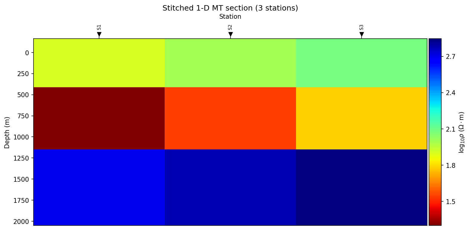
Recovered section, plotted with pycsamt.inversion.plot.plot_model().#

16.14.6. True 2-D Forward Response Handoff#

When you use MT2DForward, the response is produced by a 2-D forward solver and the TE/TM arrays are stored with frequency as the first dimension. For the inversion profile API, transpose the selected component.

>>> import numpy as np

>>> from pycsamt.forward import Grid2D, MT2DForward
>>> from pycsamt.inversion import InversionConfig, InversionWorkflow, StartingModel

>>> freqs = np.array([1.0, 10.0])

>>> grid = Grid2D.halfspace(
...     rho=100.0,
...     nx=2,
...     nz=2,
...     x_max=1000.0,
...     z_max=1000.0,
...     n_pad=0,
...     n_stations=2,
... )

>>> response = MT2DForward(freqs, grid, verbose=False).run()

>>> cfg = InversionConfig(
...     method="mt",
...     dimension="2d",
...     backend="builtin",
...     data={
...         "freqs": freqs,
...         "rho_a": response.rho_a_te.T,
...         "phase": response.phase_te.T,
...         "station_x": [0.0, 1000.0],
...         "station_names": ["S1", "S2"],
...     },
...     n_layers=2,
...     starting_model=StartingModel(
...         resistivities=[100.0, 100.0],
...         thicknesses=[500.0],
...     ),
...     max_iter=1,
...     backend_options={
...         "profile_mode": "fd2d",
...         "nx": 2,
...         "n_pad": 0,
...         "x_margin": 0.0,
...         "x_max": 1000.0,
...         "components": ("te",),
...         "regularization_weight": 0.0,
...         "forward_verbose": False,
...     },
... )

>>> result = InversionWorkflow(cfg).run()

>>> print(result.summary())
InversionResult(method='mt', dimension='2d', backend='builtin', status='converged', rms=0)

This example is intentionally small – a 2x2 halfspace grid started from the halfspace itself, so a single iteration already fits exactly. It demonstrates the data contract and the profile_mode="fd2d" option without making the documentation build depend on a large numerical run. For production studies, increase the grid resolution, station count, frequency coverage, padding, and regularization with care.

16.14.7. Backend Choice After Forward Tests#

Use the forward experiment to decide which inverse backend is appropriate.

Forward experiment	Good first inversion target	When to move to a larger backend
1-D layered MT, AMT, or CSAMT	`backend="builtin"` with `dimension="1d"`.	Move to `simpeg` or `pygimli` when you need optional external physics, meshing, or regularization features.
1-D TEM	`backend="builtin"` with `method="tdem"`.	Move to `pygimli` when your workflow requires its TDEM tools.
Station-by-station profile	`backend="builtin"` with `dimension="2d"`.	Move to `occam2d` when lateral 2-D physics and native Occam2D files are required.
2-D MT finite-difference test	Built-in finite-difference profile mode for compact experiments.	Move to Occam2D, MARE2DEM, or a specialized workflow for production 2-D inversion.
Quasi-3-D forward grid	Use for survey design, sensitivity, and synthetic catalogue creation.	Move to `modem` when a native 3-D inversion dataset and mesh are required (see ModEM).

External backends are lifecycle adapters. They may prepare and validate native files without launching an executable. Use run_external=True only after the command, files, paths, and licensing/runtime environment have been reviewed.

16.14.8. Error Model Handoff#

The error model is the most common source of misleading synthetic recovery tests. A recovery that succeeds with unrealistically small noise does not prove that a field inversion will resolve the same target.

Use these rules:

Match error_floor to the relative noise applied to apparent resistivity.
Match phase_error to the expected absolute phase uncertainty in degrees.
Keep the random seed used to generate synthetic noise.
Store whether the noise is independent, frequency-dependent, station-based, or field-realistic.
Do not tune the error floor only to force a visually pleasing model.
Compare the predicted response with the noisy data and the clean data.

The inversion objective weights residuals by the supplied data uncertainty – the same \(W_d\) and forward operator \(F(m)\) from (2) and (1), just written out as a residual vector rather than squared into a scalar objective:

(3)#\[r = W_d \left( d_{\mathrm{obs}} - F(m) \right).\]

If \(W_d\) is too strong because uncertainties are too small, the inversion may chase noise. If \(W_d\) is too weak because uncertainties are too large, the inversion may stop at an oversmoothed model. The rms values printed throughout this page are exactly this residual, reduced to a single RMS misfit number – close to 1 is the target, not as close to 0 as possible.

16.14.9. What To Compare#

For a synthetic recovery test, compare four things.

Model recovery: Does the recovered model place the main conductive or resistive target in the correct depth and lateral position? Exact layer values are less important than recoverable structure.
Data recovery: Does the predicted response fit the noisy observations within the intended uncertainty, giving an RMS misfit near 1? A beautiful model with poor residuals is not a successful inversion.
Sensitivity: Is the recovered feature inside the depth and frequency range to which the survey is sensitive? Low-confidence deep features should not be interpreted as resolved geology.
Stability: Does the result remain broadly consistent when the starting model, regularization, noise seed, or station spacing changes?

Archive each recovery experiment with enough metadata to reproduce it later:

recovery_experiment/
  config.toml
  truth_model.json
  forward_response.npz
  noisy_response.npz
  inversion_result.npz
  model.csv
  diagnostics.json
  notes.md

This archive pattern is especially useful when forward modelling is used to justify acquisition design or inversion parameter choices in a report.

16.14.10. Common Failure Modes#

The clean synthetic recovers, but the noisy synthetic does not.: The target may be below the practical resolution of the survey. Revisit frequency range, station spacing, source geometry, and error floors.
The response changes, but the inversion cannot place the target.: The data may be sensitive to the target without being able to localize it under the chosen parameterization. Try a simpler target, a different starting model, or a backend with more suitable dimensionality.
The stitched 2-D section looks plausible but disagrees with a 2-D forward test.: Lateral currents or off-station structure may be important. Use native 2-D inversion rather than interpreting stitched 1-D columns as true 2-D physics.
The inversion changes strongly when the starting model changes.: The problem is non-unique or underconstrained. Increase prior information, simplify the model, or report the range of acceptable models instead of a single image.
A quasi-3-D forward response is treated as a production 3-D inversion file.: Quasi-3-D responses are valuable for testing and survey design, but native ModEM-style inversion requires proper station data, mesh, covariance/error definitions, and executable-specific files.

16.14.11. Recommended Workflow#

Use this sequence before a field inversion:

Run a halfspace forward model and confirm that the response units and axes are correct.
Add one target layer or block and confirm that the response changes in the expected frequency or time range.
Add realistic noise and invert the synthetic data.
Repeat with a starting model that is deliberately imperfect.
Repeat with a target near the expected resolution limit.
Select the backend only after the recovery tests show which dimensionality and parameterization are justified.
Archive the forward response, inversion configuration, result, and diagnostics.

Useful next pages: