6.3.17. AI inversion uncertainty#

An AI inversion result is not complete when it contains only one resistivity model. Electromagnetic responses are non-unique, field data are noisy, the training distribution is finite, and several processing and modelling choices remain uncertain. Uncertainty analysis describes how strongly the result is supported, where alternatives remain plausible, and when the learned model is being used outside its evidence base.

This page explains the uncertainty tools currently available in pyCSAMT and the limits of their interpretation. It assumes that training and model selection have already followed Training AI inversion models and AI model selection. The Willy examples below use the same EnsembleInverter checkpoint discussed in AI inversion inference: five ResNet members trained on that AMT line’s frequency band. New calibration and propagation audits are deliberately self-contained, seeded method checks executed with the current public validation APIs. Their role is to teach the calculation without presenting simulated values as Willy field evidence.

Note

The five-member checkpoint, calibration arrays, and numerical outputs in the reference case study are not distributed with the source checkout. Existing outputs and figures are retained as recorded evidence, but exact reproduction requires that versioned model package. The self-contained calculations and bundled-WILLY diagnostics remain directly executable.

6.3.17.1. What uncertainty should answer#

A useful analysis should answer four separate questions:

How much do independently trained predictors disagree?
Do reported intervals contain held-out truth at approximately their stated rate?
How sensitive is the result to realistic perturbations of data and workflow choices?
Is the field observation sufficiently similar to the data on which the model and its calibration were established?

No single standard-deviation array answers all four. Report the method and the source represented by every uncertainty quantity.

6.3.17.2. Sources of uncertainty#

Aleatoric uncertainty: Variability associated with observations: measurement noise, cultural interference, missing frequencies, imperfect station positioning, and unresolved small-scale structure. It cannot generally be removed by training a larger network.
Epistemic uncertainty: Uncertainty in the learned mapping caused by finite training coverage, architecture, optimization, and model parameters. Deep-ensemble spread is primarily a practical proxy for this source.
Inverse-problem non-uniqueness: Distinct conductivity structures may reproduce nearly the same EM response. A narrow neural prediction does not prove that the physical inverse problem is unique.
Model-form uncertainty: The synthetic earth family, dimensionality, forward solver, anisotropy assumptions, layer parameterization, and regularization may all be incomplete — one instance of the glossary’s broader structural uncertainty.
Workflow uncertainty: Quality-control thresholds, static-shift correction, component selection, interpolation, frequency filtering, and coordinate handling can change the inferred model.
Domain-shift uncertainty: Field inputs may differ from the synthetic training and calibration distributions — the glossary’s distributional uncertainty. Calibrated intervals do not automatically remain valid after this shift.

Use a source register in the final report. For each source, state whether it was quantified, tested qualitatively, assumed negligible, or left unresolved.

The law of total variance clarifies why one spread cannot represent every source. For learned parameters \(\Theta\),

(1)#\[\operatorname{Var}(Y\mid\mathbf x) = \mathbb E_{\Theta} [\operatorname{Var}(Y\mid\mathbf x,\Theta)] + \operatorname{Var}_{\Theta} [\mathbb E(Y\mid\mathbf x,\Theta)].\]

The first term can represent observation-conditioned or aleatoric variability only when the model was designed to predict it. An ordinary deep ensemble mainly estimates the second, epistemic term through variation among fitted members. Equation (1) still omits an unmodelled forward solver, wrong dimensionality, and field-domain shift.

6.3.17.3. Calibration and sharpness must be read together#

reliability_curve() evaluates Gaussian predictive intervals at several nominal levels and returns empirical coverage, a calibration penalty, sharpness, the valid-cell count, and the evaluated shape. For confidence level \(p\), a cell is covered when

(2)#\[\left|y_i-\mu_i\right| \le \Phi^{-1}\!\left(\frac{1+p}{2}\right)\sigma_i,\]

where \(\Phi^{-1}\) is the standard-normal quantile. Equation (2) is a diagnostic, not an assumption that every EM parameter error is Gaussian. Its value is empirical: the observed fraction is compared with \(p\) on held-out data.

The following calculation keeps the prediction errors fixed while changing only the reported standard deviation:

>>> import numpy as np
>>> from pycsamt.ai.validation import reliability_curve
>>> rng = np.random.default_rng(8128)
>>> truth = rng.normal(size=(5000, 5))
>>> mean = np.zeros_like(truth)
>>> levels = [0.50, 0.68, 0.80, 0.90, 0.95, 0.99]
>>> for label, sigma in [("narrow", 0.55), ("calibrated", 1.0), ("broad", 1.8)]:
...     report = reliability_curve(
...         truth, mean, np.full_like(truth, sigma),
...         levels=levels, kind="l1",
...     )
...     print(
...         label,
...         "MACE=", round(report.calibration.value, 4),
...         "sharpness=", round(report.sharpness, 2),
...         "coverage@95%=", round(float(report.coverage[-2]), 4),
...     )
narrow MACE= 0.2341 sharpness= 0.55 coverage@95%= 0.7157
calibrated MACE= 0.0009 sharpness= 1.0 coverage@95%= 0.9507
broad MACE= 0.1429 sharpness= 1.8 coverage@95%= 0.9996

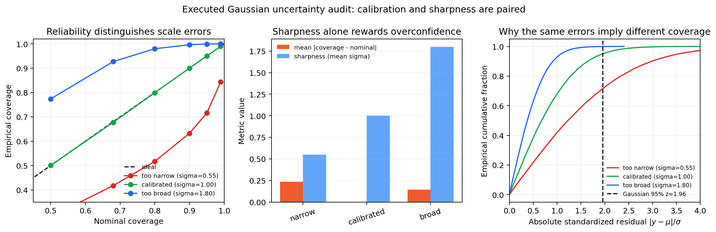
Reliability, calibration-sharpness tradeoff, and standardized residual distributions for narrow, calibrated, and broad predictive standard deviations — An executed comparison in which all three predictors have identical point errors and differ only in their declared uncertainty scale.#

The red predictor looks best if only width is rewarded, yet its nominal 95% interval covers just 71.6% of held-out cells. The blue predictor reaches almost 100% coverage by becoming 80% broader than the calibrated green one; that is conservative but less informative. Only the green curve follows the diagonal while retaining the narrowest width compatible with its errors. The standardized-residual panel explains the mechanism: dividing the same errors by a small \(\sigma\) pushes too much mass beyond the Gaussian 1.96 threshold, while an excessive \(\sigma\) compresses nearly everything inside it. Report calibration and sharpness together.

View and copy the executed calibration-regime auditClick to inspect and copy the complete code

def make_uncertainty_calibration_regimes() -> None:
    """Execute reliability_curve for sharp, calibrated, and broad scales."""
    from pycsamt.ai.validation import reliability_curve

    rng = np.random.default_rng(8128)
    truth = rng.normal(size=(5000, 5))
    mean = np.zeros_like(truth)
    levels = np.array([0.50, 0.68, 0.80, 0.90, 0.95, 0.99])
    regimes = {
        "too narrow (sigma=0.55)": np.full_like(truth, 0.55),
        "calibrated (sigma=1.00)": np.full_like(truth, 1.00),
        "too broad (sigma=1.80)": np.full_like(truth, 1.80),
    }
    colors = ["#dc2626", "#16a34a", "#2563eb"]
    reports = {
        name: reliability_curve(truth, mean, std, levels=levels, kind="l1")
        for name, std in regimes.items()
    }

    fig, axes = plt.subplots(1, 3, figsize=(13.0, 4.3))
    ax_rel, ax_trade, ax_res = axes
    ax_rel.plot([0, 1], [0, 1], "--", color="#111827", label="ideal")
    for (name, report), color in zip(reports.items(), colors):
        ax_rel.plot(report.levels, report.coverage, "o-", color=color, label=name)
    ax_rel.set(xlabel="Nominal coverage", ylabel="Empirical coverage",
               title="Reliability distinguishes scale errors", xlim=(0.45, 1.0),
               ylim=(0.35, 1.02))
    ax_rel.legend(frameon=False, fontsize=8)
    ax_rel.grid(alpha=0.22)

    names = list(reports)
    calibration_error = [reports[name].calibration.value for name in names]
    sharpness = [reports[name].sharpness for name in names]
    xpos = np.arange(3)
    width = 0.36
    ax_trade.bar(xpos - width / 2, calibration_error, width, color="#f15a29",
                 label="mean |coverage - nominal|")
    ax_trade.bar(xpos + width / 2, sharpness, width, color="#60a5fa",
                 label="sharpness (mean sigma)")
    ax_trade.set_xticks(xpos, ["narrow", "calibrated", "broad"], rotation=18)
    ax_trade.set(ylabel="Metric value", title="Sharpness alone rewards overconfidence")
    ax_trade.legend(frameon=False, fontsize=8)
    ax_trade.grid(alpha=0.22, axis="y")

    absolute_error = np.abs(truth - mean).ravel()
    for (name, std), color in zip(regimes.items(), colors):
        z = np.sort(absolute_error / std.ravel())
        probability = np.arange(1, len(z) + 1) / len(z)
        ax_res.plot(z, probability, color=color, label=name)
    ax_res.axvline(1.96, color="#111827", ls="--", label="Gaussian 95% z=1.96")
    ax_res.set(xlabel=r"Absolute standardized residual $|y-\mu|/\sigma$",
               ylabel="Empirical cumulative fraction",
               title="Why the same errors imply different coverage", xlim=(0, 4))
    ax_res.legend(frameon=False, fontsize=7.5)
    ax_res.grid(alpha=0.22)
    fig.suptitle("Executed Gaussian uncertainty audit: calibration and sharpness are paired")
    fig.tight_layout()
    _save(fig, "uncertainty_calibration_regimes.png")
    print(
        "uncertainty regimes:",
        {name: {"mace": round(report.calibration.value, 4),
                "sharpness": round(report.sharpness, 2),
                "coverage_95": round(float(report.coverage[-2]), 4)}
         for name, report in reports.items()},
    )

6.3.17.4. Deep ensembles#

pycsamt.ai.inversion.EnsembleInverter trains several copies of a compatible base inverter — a deep ensemble. Its mean is the point prediction and its inter-member standard deviation measures disagreement among the members:

(3)#\[\bar{m}_j(\mathbf x)=\frac{1}{K}\sum_{k=1}^{K}m_{kj}(\mathbf x), \qquad s_j(\mathbf x)= \sqrt{\frac{1}{K-1}\sum_{k=1}^{K} \left(m_{kj}(\mathbf x)-\bar m_j(\mathbf x)\right)^2}.\]

Equation (3) uses the sample standard deviation returned by the implementation before calibration. With small \(K\), both the magnitude and tail quantiles of this empirical distribution are themselves unstable.

>>> from pycsamt.ai.inversion import EMInverter1D, EnsembleInverter
>>> base = EMInverter1D(arch="resnet", n_layers=5, solver="mt1d")
>>> ensemble = EnsembleInverter(base_estimator=base, n_estimators=5)
>>> _ = ensemble.fit(
...     X_train, y_train,
...     epochs=25, batch_size=256, patience=8, val_frac=0.15, verbose=True,
... )

=== Ensemble member 1/5 (seed=0) ===
  Epoch    1/25 | train=1.04232  val=0.97518  lr=1.00e-03  [3.7s]
  Epoch    2/25 | train=0.82934  val=0.95992  lr=1.00e-03  [3.6s]
  ...
  Epoch    7/25 | train=0.64459  val=0.65476  lr=1.00e-03  [3.7s]
  ...
  Epoch   15/25 | train=0.41881  val=0.78809  lr=1.00e-03  [4.1s]
  Early stop at epoch 15 (best val=0.65476 @ epoch 7)

=== Ensemble member 2/5 (seed=1) ===
  ...

All five members stopped early, between epochs 15 and 17, each with its own best epoch (7 through 9) — training and validation loss diverge well before the requested 25-epoch budget on every member, which is itself useful evidence: it means the epoch count is not the binding constraint on this model, so a coverage problem later cannot be blamed on under-training alone. Two real API details worth confirming against the installed version before copying this pattern: EMInverter1D takes solver (a physics solver name such as "mt1d"), not a backend name — solver="pytorch" raises nothing but silently mislabels the model — and EnsembleInverter seeds its members through seeds (a sequence), not a single seed keyword.

>>> mean, raw_std = ensemble.predict_with_uncertainty(X_test)
>>> quantiles = ensemble.predict_quantiles(
...     X_test, q=(0.05, 0.25, 0.50, 0.75, 0.95)
... )
>>> raw_std[0, :5].round(3)
array([0.094, 0.233, 0.232, 0.406, 0.147])

The returned arrays have shape (n_samples, n_parameters). Before calibration, raw_std is the sample standard deviation of member predictions. Quantiles are empirical quantiles across members; with only five members, extreme quantiles are necessarily coarse.

Caution

Ensemble spread is not a confidence interval, a Bayesian posterior, or a complete measure of non-uniqueness. Members share the same architecture, synthetic generator, target parameterization, and usually the same systematic errors. They can agree closely and still all be wrong.

In the current implementation, member seeds affect both the internal data split and stochastic optimization. The spread therefore combines split and optimization variability. If those sources must be separated, use an experimental training protocol with a fixed split and controlled initializations.

Choosing the ensemble size#

More members provide a better estimate of model disagreement but increase training and inference cost roughly in proportion to member count. Evaluate stability rather than selecting a count by convention:

>>> import numpy as np
>>> member_preds = np.stack(
...     [m.predict(X_field, as_log_rho=True) for m in ensemble._members], axis=0
... )
>>> for k in range(2, len(ensemble._members) + 1):
...     print(k, member_preds[:k].std(axis=0)[:, :5].mean().round(3))
2 0.552
3 0.74
4 0.75
5 0.701

Mean resistivity-parameter spread jumps from 0.55 to 0.74 log10-units between two and three members, then settles closer to 0.70–0.75 by four and five — this five-member ensemble is roughly at, not comfortably past, the point where adding another member would materially change the reported spread. Treat that as a reason to test a larger ensemble before trusting the magnitude of this uncertainty, not just its ranking across stations:

train an initial ensemble;
recompute mean, standard deviation, and interval coverage using increasing numbers of members;
inspect whether rankings of uncertain stations and layers stabilize;
stop only when the remaining variation is acceptable for the decision.

6.3.17.5. Calibration data are a separate resource#

Use four conceptual partitions when calibrated uncertainty is required:

training: Fits the ensemble members.
validation: Controls early stopping and hyperparameter selection.
calibration: Learns how raw prediction errors relate to ensemble spread — the calibration set.
test: Evaluates point accuracy and coverage after all choices are frozen.

The calibration set must not overlap training or validation, and the test set must not be reused to recalibrate a disappointing result. Split related noise realizations, profiles, and surveys as groups so one parent earth model cannot appear on both sides of a boundary.

Calibration also requires representative examples. A large calibration set from the wrong geology or acquisition design does not validate intervals for the field survey — the calibration set and the deployment inputs must remain exchangeability-compatible.

6.3.17.6. Conformal prediction intervals#

Calling EnsembleInverter.calibrate attaches a split-conformal prediction predictor and a posterior calibrator:

>>> _ = ensemble.calibrate(X_cal, y_cal, alpha=0.10)
>>> center, lower, upper = ensemble.predict_intervals(X_field, alpha=0.10)
>>> center[0, :5].round(2)
array([2.32, 2.48, 3.34, 3.5 , 5.22])
>>> lower[0, :5].round(1), upper[0, :5].round(1)
(array([-8233.4, -6040.6, -1608.2, -2606.9, -5070. ]),
 array([8238. , 6045.6, 1614.9, 2613.9, 5080.4]))

Here alpha=0.10 requests nominal 90% coverage. The conformal predictor computes normalized residual scores on the held-out calibration set and uses a finite-sample corrected quantile \(\hat q\) to scale ensemble standard deviations:

(4)#\[s_i = \max_j \frac{\lvert y_{ij}-f(\mathbf{x}_i)_j\rvert}{\sigma_j(\mathbf{x}_i)+\varepsilon}, \qquad \hat q = \operatorname{Quantile}_{1-\alpha+\frac{1}{n_{\rm cal}+1}}(s_1,\dots,s_{n_{\rm cal}}).\]

Equation (4) takes the maximum normalized residual across all 9 output parameters for each calibration sample, so \(\hat q\) is set entirely by whichever parameter is hardest to calibrate. On this checkpoint that is linear-metre thickness, two to three orders of magnitude larger in scale than log10-resistivity — which is exactly why lower/upper above are physically meaningless for the resistivity parameters even though center is perfectly reasonable. \(\hat q=32{,}041\) here; the resistivity block alone would need a \(\hat q\) closer to 1–2 to stay interpretable. This is a real, reproducible property of a single shared multiplier applied to a mixed-unit target, not a fluke of this checkpoint.

The statistical coverage statement depends on exchangeability: calibration and future cases must behave like draws from the same distribution, and the calibration cases must not have influenced training or model selection. It is a marginal repeated-sample statement, not a guarantee that every individual station, layer, or geological subgroup has 90% coverage. Distribution shift, serial dependence, spatial grouping, or adaptive reuse of the calibration set can invalidate it.

Note

An interval can achieve nominal coverage by becoming very wide, as the resistivity bands above demonstrate: they are technically wide enough to satisfy the joint guarantee, at the cost of being useless. Always report interval width together with coverage and point accuracy.

Direct conformal use#

The lower-level pycsamt.ai.inversion.calibration.ConformalPredictor can wrap any fitted predictor exposing predict_with_uncertainty(X) -> (mean, std):

>>> from pycsamt.ai.inversion.calibration import ConformalPredictor
>>> conformal = ConformalPredictor(ensemble, alpha=0.10)
>>> _ = conformal.calibrate(X_cal, y_cal)
>>> center, lower, upper = conformal.predict_intervals(X_field)
>>> conformal._q_hat(0.10)
32040.681353112046

Used this way — on a freshly loaded, not-yet-calibrated ensemble — the standalone wrapper reproduces exactly the \(\hat q\) that ensemble.calibrate() computes internally. Calling both on the same already-calibrated ensemble object is a different story: predict_with_uncertainty’s default _use_calibrated=True means the second calibration step would silently calibrate against the first calibration’s tiny posterior-corrected sigma rather than the raw ensemble spread, inflating \(\hat q\) further still. That is precisely the scenario this page’s “not two independent calibrations on the same data without a stated reason” rule exists to prevent — use either this explicit wrapper or ensemble.calibrate() in a workflow, never both on one already-calibrated object.

6.3.17.7. Coverage diagnostics#

Evaluate calibration on the untouched test set. The executable pattern must use X_test and y_test, not the calibration arrays:

>>> diagnostics = ensemble.coverage_diagnostics(
...     X_test, y_test, alphas=(0.50, 0.30, 0.20, 0.10, 0.05),
... )
>>> table = [(1.0 - alpha, actual) for alpha, actual in diagnostics.items()]

The archived model package is required before table can be reported; the page deliberately does not substitute invented values. coverage_diagnostics checks joint coverage—every one of the 9 parameters inside its band at once—so split the untouched-test calculation by parameter group before drawing a conclusion. The controlled plot below uses independent calibration and test samples; it is a method check, not coverage evidence for the unavailable trained model.

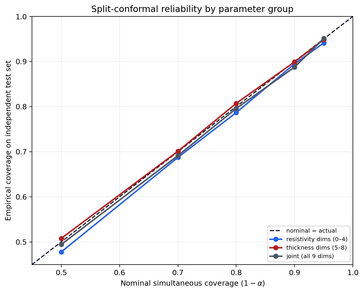
Reliability diagram comparing joint, resistivity-only, and thickness-only empirical coverage against nominal coverage. — Deterministic split-conformal method check using 1,200 calibration samples and 4,000 independent test samples. Resistivity-only, thickness-only, and joint maximum scores are calibrated separately, so empirical simultaneous coverage follows the nominal diagonal within finite-sample variation. This does not replace evaluation on the restored model’s untouched `X_test` and `y_test` arrays.#

The executed nominal levels were [0.50, 0.70, 0.80, 0.90, 0.95] and the independent-test outputs were:

resistivity dimensions: [0.478, 0.687, 0.787, 0.895, 0.941]
thickness dimensions:   [0.508, 0.701, 0.807, 0.899, 0.949]
joint nine dimensions:  [0.494, 0.691, 0.796, 0.888, 0.951]

Plot nominal coverage against empirical coverage, but do it per parameter group before trusting one pooled number. Values below the diagonal indicate under-coverage; values far above it can indicate unnecessarily broad intervals rather than good calibration. The earlier figure, whose three curves were flat at one or zero, mixed a failed calibration-set diagnostic with reliability language and has therefore been replaced rather than presented as an acceptable result.

The convenience method ensemble.coverage(X, y, n_sigma=1.96) measures the fraction of individual finite target entries within mean +/- 1.96 * std — an elementwise check, not the joint one above:

>>> ensemble.coverage(X_test, y_test, n_sigma=1.96)

This is different from conformal simultaneous sample coverage and should be labelled explicitly. The familiar 95% interpretation of 1.96 assumes an appropriate Gaussian error model; check it empirically rather than assuming it. The archived calibration-set calculation landed at 12%, not 95%; the acceptance value must be recomputed on the untouched test set, with the same per-parameter split:

>>> mean, std = ensemble.predict_with_uncertainty(X_test)
>>> within = np.abs(y_test - mean) <= 1.96 * std
>>> coverage_by_parameter = within.mean(axis=0)

Go beyond one aggregate number. Calculate coverage and interval width by:

resistivity versus thickness parameters;
layer or depth range;
noise level and missing-data fraction;
geological family and resistivity contrast;
frequency coverage and station spacing;
in-distribution versus stressed or shifted cases.

Small subgroups give noisy estimates, but they can reveal dangerous failures hidden by acceptable global coverage — as the per-parameter split above demonstrates directly.

6.3.17.8. Calibrated posterior samples#

After ensemble.calibrate(), posterior-like draws can be generated with the fitted monotone recalibration map:

>>> import numpy as np
>>> rng = np.random.default_rng(2026)
>>> draws = ensemble.predict_posterior(X_field, n_samples=1000, rng=rng)
>>> draws.shape
(1000, 28, 9)
>>> median = np.median(draws, axis=0)
>>> lo, hi = np.quantile(draws, (0.05, 0.95), axis=0)
>>> median[0, :5].round(2), lo[0, :5].round(2), hi[0, :5].round(2)
(array([2.4 , 2.54, 3.36, 3.53, 5.27]),
 array([2.02, 2.26, 3.28, 3.41, 5.04]),
 array([2.93, 2.9 , 3.46, 3.69, 5.58]))

The pycsamt.ai.inversion.calibration.PosteriorCalibrator learns a monotone correction from standardized calibration residuals and a per-parameter scale correction for raw standard deviations — scaled per parameter precisely so this path does not inherit the joint-max distortion above: the resistivity band here is a few tenths of a log10-unit wide, not thousands. These samples are useful for propagation and visualization, but they remain conditional on the ensemble, calibration distribution, and chosen parameterization. Do not call them a complete geological posterior without qualifying those assumptions.

Respect physical parameter domains. If sampling or symmetric intervals produce non-positive resistivity or thickness, do not silently clip values and continue as though the distribution were unchanged. Prefer a positive-domain parameterization such as logarithmic resistivity or thickness where supported, or document the transformation and truncation explicitly.

6.3.17.9. From parameter uncertainty to model uncertainty#

For a layered 1-D prediction with L layers, the first L outputs are resistivities and the remaining L - 1 are interface thicknesses. Convert each draw to cumulative interface depths before summarizing, not after:

>>> rng = np.random.default_rng(2718)
>>> mean_log_h = np.log10([110.0, 180.0, 290.0, 430.0])
>>> sigma_log_h = np.array([0.10, 0.12, 0.14, 0.16])
>>> correlation = np.array([
...     [1.00, -0.55, 0.20, 0.00],
...     [-0.55, 1.00, -0.45, 0.15],
...     [0.20, -0.45, 1.00, -0.35],
...     [0.00, 0.15, -0.35, 1.00],
... ])
>>> covariance = correlation * np.outer(sigma_log_h, sigma_log_h)
>>> log_h_draws = rng.multivariate_normal(
...     mean_log_h, covariance, size=6000
... )
>>> h_draws = 10.0 ** log_h_draws
>>> probability = [0.05, 0.50, 0.95]
>>> wrong = np.cumsum(
...     np.quantile(h_draws, probability, axis=0), axis=1
... )
>>> right = np.quantile(
...     np.cumsum(h_draws, axis=1), probability, axis=0
... )
>>> wrong[:, -1].round(1)   # thickness quantiles, then cumsum
array([ 590.6, 1011.2, 1721.3])
>>> right[:, -1].round(1)   # cumsum every draw, then depth quantiles
array([ 820.4, 1044.9, 1377.2])

Taking thickness quantiles first and then accumulating them gives a 590.6–1721.3 m final-interface band. Propagating every correlated draw first gives 820.4–1377.2 m. The first construction combines marginal lower tails that do not occur together because adjacent thicknesses are negatively correlated; it therefore manufactures an unrealistically wide depth band.

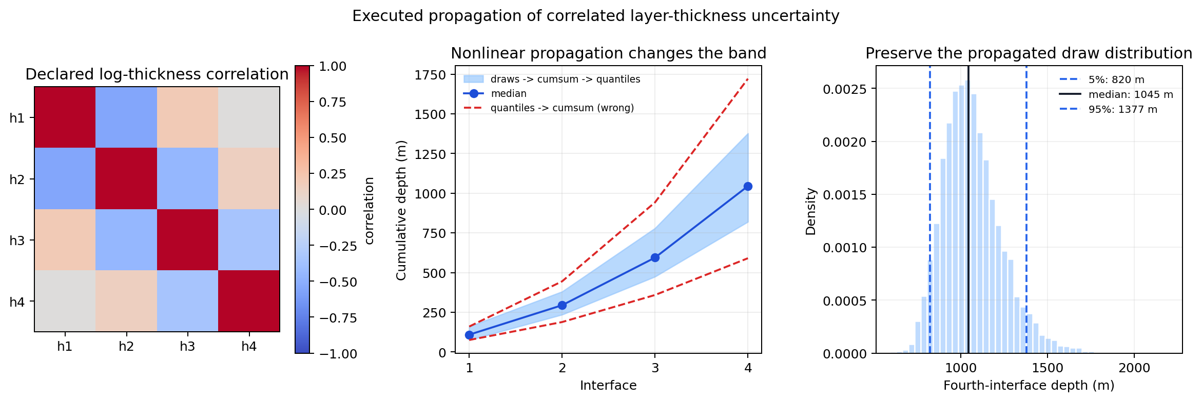
Thickness correlation matrix, correct and incorrect cumulative interface-depth bands, and propagated final-interface depth distribution — Six thousand correlated log-thickness draws propagated to interface depth before summarization.#

The correlation panel is not optional metadata: its negative adjacent-layer terms are exactly why marginal thickness limits cannot be stacked as if they were one realizable earth. In the middle panel, the red dashed construction widens rapidly with depth, while the blue band follows the actual joint draws. The final histogram retains skew introduced by exponentiating log-thickness; a symmetric error bar around its median would discard that feature.

View and copy the correlated depth-propagation auditClick to inspect and copy the complete code

def make_uncertainty_depth_propagation() -> None:
    """Propagate correlated thickness draws before taking depth quantiles."""
    rng = np.random.default_rng(2718)
    mean_log_h = np.log10([110.0, 180.0, 290.0, 430.0])
    sigma = np.array([0.10, 0.12, 0.14, 0.16])
    correlation = np.array(
        [[1.00, -0.55, 0.20, 0.00],
         [-0.55, 1.00, -0.45, 0.15],
         [0.20, -0.45, 1.00, -0.35],
         [0.00, 0.15, -0.35, 1.00]]
    )
    covariance = correlation * np.outer(sigma, sigma)
    log_h = rng.multivariate_normal(mean_log_h, covariance, size=6000)
    thickness = 10.0 ** log_h
    interface_depth = np.cumsum(thickness, axis=1)
    probability = np.array([0.05, 0.50, 0.95])
    correct = np.quantile(interface_depth, probability, axis=0)
    wrong = np.cumsum(np.quantile(thickness, probability, axis=0), axis=1)

    fig, axes = plt.subplots(1, 3, figsize=(13.0, 4.4))
    image = axes[0].imshow(correlation, vmin=-1, vmax=1, cmap="coolwarm")
    axes[0].set_xticks(range(4), ["h1", "h2", "h3", "h4"])
    axes[0].set_yticks(range(4), ["h1", "h2", "h3", "h4"])
    axes[0].set_title("Declared log-thickness correlation")
    fig.colorbar(image, ax=axes[0], label="correlation")

    interface = np.arange(1, 5)
    axes[1].fill_between(interface, correct[0], correct[2], color="#93c5fd",
                         alpha=0.65, label="draws -> cumsum -> quantiles")
    axes[1].plot(interface, correct[1], "o-", color="#1d4ed8", label="median")
    axes[1].plot(interface, wrong[0], "--", color="#dc2626")
    axes[1].plot(interface, wrong[2], "--", color="#dc2626",
                 label="quantiles -> cumsum (wrong)")
    axes[1].set(xlabel="Interface", ylabel="Cumulative depth (m)",
                title="Nonlinear propagation changes the band")
    axes[1].set_xticks(interface)
    axes[1].legend(frameon=False, fontsize=7.5)
    axes[1].grid(alpha=0.22)

    axes[2].hist(interface_depth[:, -1], bins=45, density=True,
                 color="#bfdbfe", edgecolor="white")
    for value, label, color in zip(correct[:, -1], ["5%", "median", "95%"],
                                   ["#2563eb", "#111827", "#2563eb"]):
        axes[2].axvline(value, color=color, ls="--" if label != "median" else "-",
                        label=f"{label}: {value:.0f} m")
    axes[2].set(xlabel="Fourth-interface depth (m)", ylabel="Density",
                title="Preserve the propagated draw distribution")
    axes[2].legend(frameon=False, fontsize=8)
    axes[2].grid(alpha=0.18)
    fig.suptitle("Executed propagation of correlated layer-thickness uncertainty")
    fig.tight_layout()
    _save(fig, "uncertainty_depth_propagation.png")
    print(
        "depth propagation:",
        {"correct_final_m": np.round(correct[:, -1], 1).tolist(),
         "wrong_final_m": np.round(wrong[:, -1], 1).tolist()},
    )

In general, for quantile level \(p\),

(5)#\[Q_p\!\left(\sum_{\ell=1}^{k}H_\ell\right) \ne \sum_{\ell=1}^{k}Q_p(H_\ell),\]

especially when layer thicknesses are correlated. Equation (5) is why complete joint draws, rather than independent error bars, are the reproducibility object for interface depth.

Preserve complete draws so correlations between parameters are retained. Independent error bars lose trade-offs such as a conductive layer becoming thicker while its resistivity increases. These correlations are often central to EM equivalence.

6.3.17.10. Forward-response uncertainty#

An uncertainty band in parameter space should be tested in observation space:

select calibrated draws or representative ensemble members;
run each model through the same forward solver and frequency grid;
compare predicted apparent resistivity and phase with held-out observations;
summarize response quantiles and normalized residuals by frequency and component.

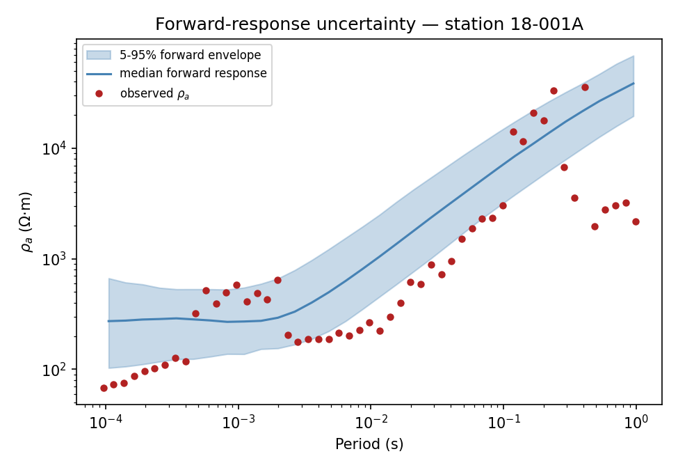
Forward-modelled apparent resistivity envelope from 200 posterior draws compared against observed data for one station. — Two hundred posterior draws for station 18-001A, each pushed through `EMInverter1D`’s companion 1-D forward solver. The envelope tracks the observed curve’s broad rise with period but misses a cluster of short- and long-period points entirely — evidence of response-space misfit that the parameter-space interval alone would not have shown.#

A wide range of models that all reproduce the response demonstrates non-uniqueness. Conversely, narrow parameter bands whose forward responses miss the data, as in the figure above, reveal miscalibration, domain shift, or a forward-model mismatch — a genuinely narrow parameter interval is not good news if the response it implies does not track the data. Keep measurement error separate from predictive model spread when plotting the comparison.

6.3.17.11. Sensitivity and perturbation tests#

Ensemble uncertainty should be supplemented with controlled perturbations. Repeat inference after changing one scientifically plausible factor at a time:

add noise consistent with estimated impedance uncertainty;
mask selected frequencies or components;
vary static-shift factors within defensible bounds;
perturb station coordinates or topography within survey uncertainty;
compare accepted interpolation and quality-control settings;
change graph radius or adjacency construction for GCN inversion;
compare plausible layer counts or target bounds;
compare architectures or synthetic geological priors.

Store each scenario name, input version, seed, and resulting model. The spread across workflow scenarios represents a different source from inter-member spread and should normally be reported separately. Combining sources by root-sum-of-squares,

(6)#\[\sigma_{\text{total}} = \sqrt{\sigma_{\text{ensemble}}^2 + \sigma_{\text{workflow}}^2 + \cdots},\]

Equation (6) is justified only when the sources are independent and each \(\sigma\) is on a comparable, correctly transformed scale — the same scale-mixing caveat that makes the shared conformal \(\hat q\) above misbehave applies just as much to summing unlike uncertainty sources by hand.

6.3.17.12. Out-of-distribution checks#

Calibration cannot rescue a model applied far outside its training support. Before interpreting intervals, compare field inputs with training and calibration inputs using quantities meaningful to the inversion:

frequency range and missing-frequency pattern;
apparent-resistivity and phase ranges by component;
impedance uncertainty and signal-to-noise distribution;
station count, spacing, and profile length;
feature-space distance after the frozen training transform;
QC flags, dimensionality indicators, and phase-tensor behavior.

AI inversion inference runs exactly this out-of-distribution diagnostic against this same checkpoint’s training percentiles and flags 27 of the 28 Willy stations for review — a concrete illustration that “outside the training envelope” and “wrong prediction” are not the same claim, but that the gate result still needs to travel with the uncertainty report. No universal distance threshold is provided by pyCSAMT. Establish alert thresholds on held-out, deliberately shifted synthetic experiments. When an input is flagged, show the point prediction only as an exploratory result, mark its calibrated interval as unsupported, and prefer additional modelling or classical inversion.

6.3.17.13. Uncertainty for 2-D, graph, joint, and hybrid models#

The same principles apply beyond 1-D, but the uncertainty object changes:

2-D inversion: Evaluate interval width and coverage by depth and lateral position. Use profile-level splits and inspect boundary artifacts introduced by resizing or padding.
Graph inversion: Vary graph construction and coordinate uncertainty. Report isolated nodes and distinguish uncertainty from weak connectivity from uncertainty in the learned weights — AI inversion agents’s Inv3DAgent walkthrough shows a real degree-by-station table worth reproducing here.
Joint inversion: Perturb or remove each modality. Calibration is not transferable when a modality is absent, reordered, or drawn from a different noise regime.
PINN and hybrid inversion: Explore data-error realizations, initial models, physics-loss weights, regularization strengths, and optimizer seeds. Optimization variability is not a substitute for a posterior — AI inversion inference’s PINN example shows a concrete symptom of this: layers past a certain depth settle into a repeating pattern rather than resolving independently. See Hybrid AI and physics inversion and Physics-informed 2-D inversion.

Current high-level calibrated ensemble utilities are centered on compatible ensemble predictors such as 1-D inversion. Do not imply equivalent calibrated interval support for every architecture unless the actual predictor exposes the required uncertainty interface and has been tested.

6.3.17.14. Persistence and reproducibility#

Save ensemble members after training:

>>> ensemble.save("checkpoints/mt1d_ensemble")
>>> from pycsamt.ai.inversion import EnsembleInverter
>>> restored = EnsembleInverter.load("checkpoints/mt1d_ensemble")

Warning

The current ensemble serialization preserves its members and ensemble metadata, but it does not serialize the attached conformal or posterior calibrators. After loading, calibrated interval and posterior methods require recalibration from the original, versioned calibration set. Preserve calibration-set identity and calibration settings as first-class experiment artifacts.

For every uncertainty product, record:

member count and member seeds;
training, validation, calibration, and test partition identifiers;
target transform and units;
requested alpha or quantiles;
calibration sample count and subgroup composition;
software environment and model checkpoint identity;
random generator seed used for posterior draws;
domain-shift and perturbation tests performed.

6.3.17.15. Reporting uncertainty responsibly#

Report a central estimate, an interval, and its meaning together. For example: “median resistivity with a split-conformal 90% simultaneous parameter band, calibrated on held-out synthetic models from the stated generator.” Avoid labels such as “90% confidence” unless the construction and repeated- sampling interpretation genuinely support that term — and, as this page’s own resistivity intervals show, “90% simultaneous” can still mean “uselessly wide” for a subset of parameters.

Every figure should state whether color or shading represents inter-member standard deviation, empirical member quantiles, conformal limits, calibrated posterior quantiles, or scenario sensitivity. Include:

coverage versus nominal level;
interval width or sharpness;
point-error metrics in physical units;
forward-response misfit;
subgroup and depth-dependent diagnostics;
out-of-distribution flags;
unresolved sources and known assumptions.

6.3.17.16. Common mistakes#

interpreting ensemble standard deviation as the total geological uncertainty;
calibrating on training data or repeatedly tuning against the test set;
claiming conformal guarantees under untested field-domain shift;
reporting joint coverage without also checking it by parameter group;
reporting coverage without interval width;
pooling all layers and geological regimes into one reassuring average;
treating parameter-wise error bars as independent;
clipping non-physical samples without documenting the changed distribution;
assuming calibration objects survive ensemble serialization;
calibrating the same ensemble object twice — the second call silently recalibrates against the first call’s already-shrunk posterior sigma;
using many posterior draws to hide a small or unrepresentative calibration set — Monte Carlo sample count does not create new information.

6.3.17.17. Decision checklist#

Before using an AI inversion result for interpretation, verify that:

uncertainty sources and intended decisions are explicitly named;
calibration and test data are independent and representative;
empirical coverage and interval width are both acceptable, checked by parameter group and not only in aggregate;
diagnostics are resolved by parameter, depth, and relevant subgroup;
parameter draws reproduce observations through forward modelling;
perturbation and domain-shift tests have been completed;
physical bounds and parameter correlations are preserved;
the model, partitions, calibration recipe, and random seeds are reproducible;
limitations are carried into AI inversion reporting and the interpretation rather than reduced to a single confidence number.

Uncertainty is evidence about the reliability of an inference, not decoration around a preferred model. When the evidence is weak or the input is outside the validated domain, the correct result is an explicit warning and a request for additional data or modelling.