11.25. Advanced EM Tools

pycsamt.emtools.advanced contains pyCSAMT’s advanced MT/AMT/CSAMT visual diagnostics. These functions are not data loaders and they are not inversion engines. They are figure-producing analysis tools that expose tensor behaviour, dimensionality, distortion, depth sensitivity, survey coherence, and station-to-station structure in ways that are difficult to see from ordinary apparent resistivity and phase curves alone.

The module is intentionally built on the same public data boundary used throughout pycsamt.emtools: every function accepts path-like inputs, EDI-like objects, or Sites containers and normalizes them with pycsamt.emtools._core.ensure_sites(). This means the examples below work with a survey directory, a list of EDI files, or a pre-loaded Sites object.

11.25.1. When To Use This Module

Use the advanced tools after basic loading and QC, when the next question is interpretive:

• Does the response behave like 1-D, 2-D, or 3-D structure?

• Are distortion indicators localized by station, period, or component?

• Which periods are likely probing the same depth interval?

• Do neighboring stations have coherent transfer-function behaviour?

• Is a proposed strike direction stable across period and method?

• Are tensor invariants, minimum-phase consistency, or phase-tensor summaries telling the same story as ordinary rho and phase plots?

The functions return matplotlib.figure.Figure objects. They do not write files by default, so scripts can save the result explicitly. The examples on this page share one loaded survey and one output directory, so later blocks build directly on sites and out defined here.

>>> from pathlib import Path
>>> from pycsamt.emtools import ensure_sites
>>> from pycsamt.emtools.advanced import plot_survey_fingerprint
>>> sites = ensure_sites(
...     "data/AMT/WILLY_DATA/L18PLT",
...     recursive=True,
...     strict=False,
...     on_dup="replace",
...     verbose=0,
... )
>>> len(list(sites))
28
>>> out = Path("results")
>>> out.mkdir(exist_ok=True)
>>> fig = plot_survey_fingerprint(sites, recursive=False)
>>> fig.savefig(out / "l18_survey_fingerprint.png", dpi=200)

ensure_sites normalizes the real 28-station L18PLT AMT line into one Sites container, so it is parsed once and reused by every example below rather than being re-read from disk each time. Every other function on this page accepts that same sites object directly.

11.25.2. Implementation Pattern

The advanced functions follow a shared implementation pattern:

1. Normalize user input with ensure_sites.

2. Iterate over stations with _iter_items and stable station names from _name.

3. Extract impedance tensor and frequency arrays with _get_z_block and, where needed, tipper arrays with _get_t_block.

4. Compute a diagnostic quantity such as rotated impedance, Bostick depth, phase-tensor skew, ellipticity, apparent anisotropy, or station-to-station correlation.

5. Render the diagnostic into Matplotlib axes.

6. Return the Figure without saving it.

Most functions expose the same input-control keywords:

recursive

Whether path-like directory inputs should be searched recursively.

on_dup

Duplicate station policy passed to ensure_sites. Use "replace" for exploratory work and "raise" for strict production checks.

strict

If True, fail when no valid site can be resolved.

verbose

Forwarded to the loading/coercion layer.

axes or ax

Optional Matplotlib axes supplied by the caller. Use these when embedding advanced diagnostics into a larger dashboard or report figure.

11.25.3. Functional Groups

Group	Functions	Main purpose
Single-station tensor diagnostics	plot_impedance_mohr_circles, plot_zt_argand, plot_rho_phase_bode, plot_apparent_resistivity_polar, plot_pt_period_clock	Inspect how one station changes with rotation, period, component, apparent resistivity, phase, and phase-tensor geometry.
Dimensionality and distortion	plot_dimensionality_ternary, plot_distortion_radar	Summarize whether responses look 1-D, 2-D, 3-D, distorted, or unstable across period and station.
Pseudosection and survey summaries	plot_sensitivity_depth_section, plot_apparent_anisotropy_section, plot_dimensionality_depth_profile, plot_z_invariants_section, plot_survey_fingerprint, plot_mt_composite_section, plot_snr_section	Convert station-period arrays into profile-style figures that expose depth sensitivity, anisotropy, invariants, SNR, and multi-metric survey structure.
Strike and coherence	plot_strike_stability_bands, plot_tf_coherence_network	Test strike stability across methods and visualize whether stations share coherent transfer-function curves.

11.25.4. Single-Station Tensor Diagnostics

These functions are best used on one station at a time, or on a survey-median summary, when you want to understand tensor behaviour before interpreting a full profile.

All five diagnostics in this block start from the complex impedance tensor

\[\begin{split}\mathbf{Z}(f) = \begin{bmatrix} Z_{xx}(f) & Z_{xy}(f) \\ Z_{yx}(f) & Z_{yy}(f) \end{bmatrix}.\end{split}\]

When a function studies rotation, pyCSAMT uses

\[\begin{split}\mathbf{Z}_\theta(f) = \mathbf{R}(\theta)\, \mathbf{Z}(f)\, \mathbf{R}(\theta)^T, \qquad \mathbf{R}(\theta) = \begin{bmatrix} \cos\theta & \sin\theta \\ -\sin\theta & \cos\theta \end{bmatrix}.\end{split}\]

Impedance Mohr circle diagrams ask how the tensor changes under every rotation. Argand diagram trajectories ask how the complex value itself moves with period. Bode consistency plots ask whether phase is consistent with the resistivity slope. Polar diagrams ask how resistivity changes with rotation direction. The phase-tensor clock asks whether tensor orientation and ellipticity remain stable with period.

>>> from pycsamt.emtools.advanced import (
...     plot_impedance_mohr_circles,
...     plot_zt_argand,
...     plot_rho_phase_bode,
...     plot_apparent_resistivity_polar,
...     plot_pt_period_clock,
... )
>>> fig_mohr = plot_impedance_mohr_circles(sites, station="18-001A")
>>> fig_argand = plot_zt_argand(sites, station="18-001A", components=("xy", "yx"))
>>> fig_bode = plot_rho_phase_bode(sites, station="18-001A", component="xy")
>>> fig_polar = plot_apparent_resistivity_polar(sites, station="18-001A")
>>> fig_clock = plot_pt_period_clock(sites, n_rings=6)

Mohr circles, Argand trajectories, and Bode plots all read left to right as a wide, period-colored curve, so they line up naturally in one three-column row:

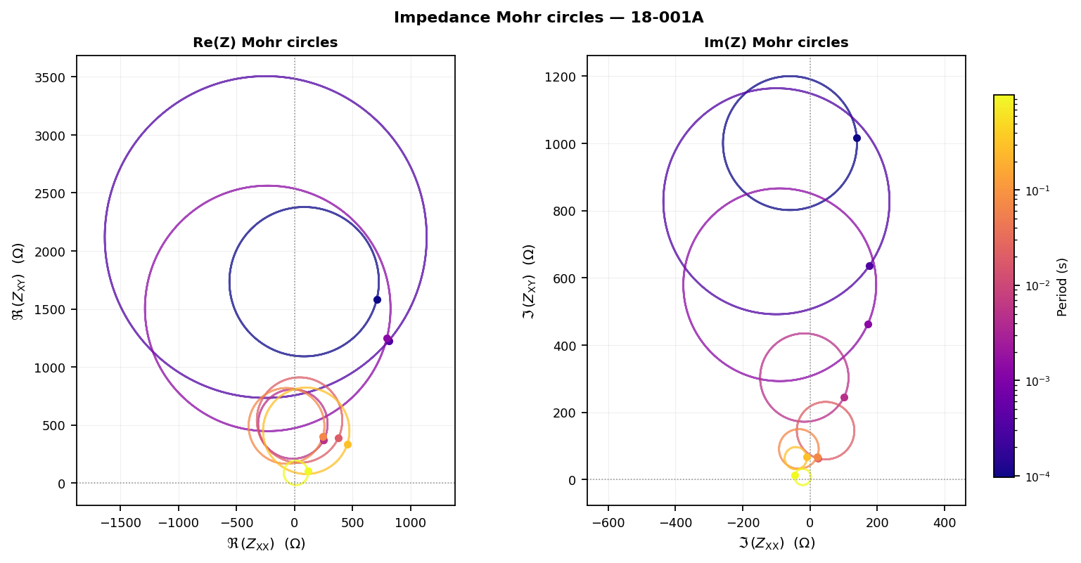
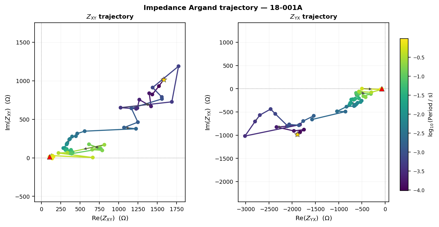
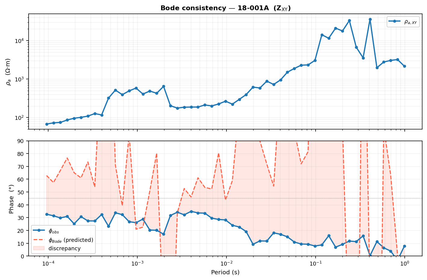
Mohr circles rotate the impedance tensor through all angles and show whether the rotated trajectories collapse to points, pass through the origin, or remain offset. Argand trajectories keep the complex impedance itself in view and use period as the trajectory parameter. Bode plots compare observed phase against the phase implied by local log(rho_a) slope.

The polar apparent-resistivity diagram and the phase-tensor period clock are both naturally square, radial figures, so they read better as their own two-column row rather than being squeezed beside the wide panels above:

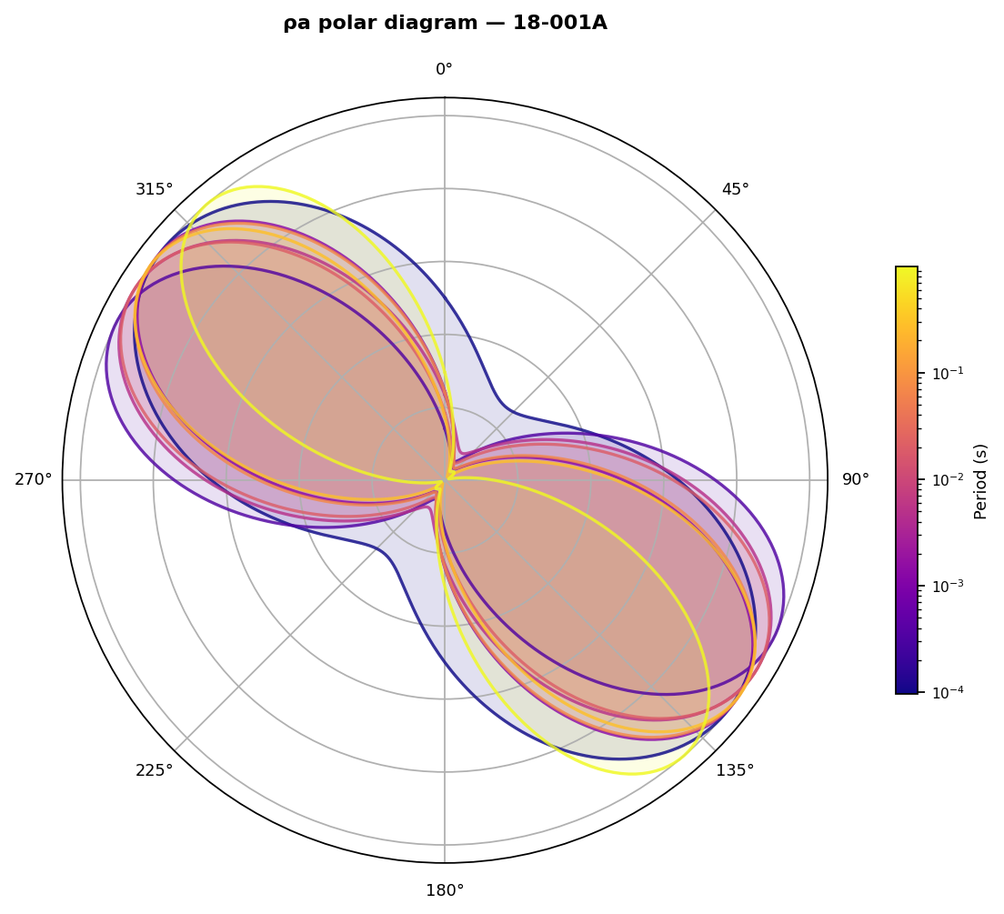
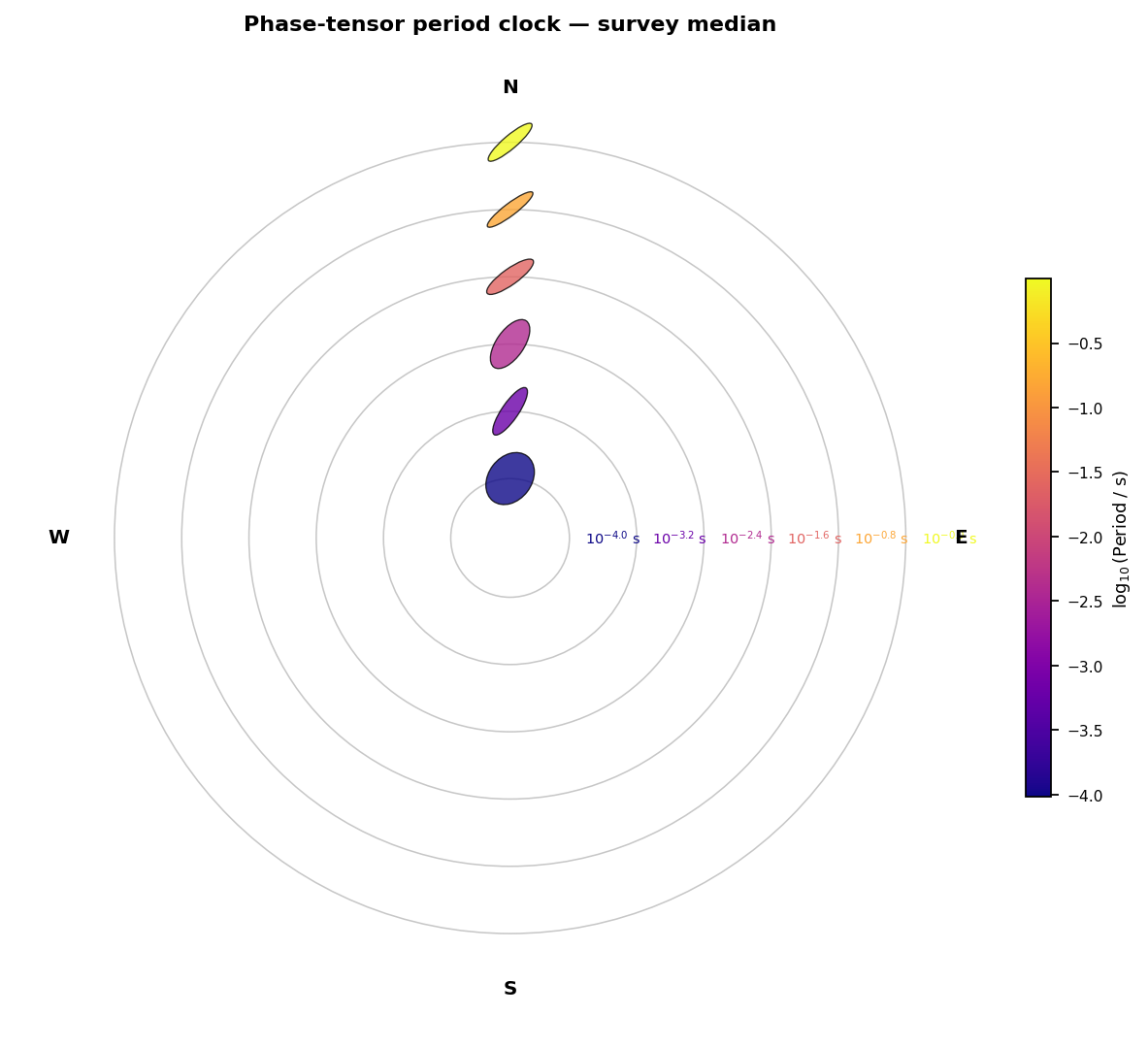
The polar plot shows how rho_a varies with rotation angle as one petal per period, and the phase-tensor period clock compresses period-dependent phase-tensor ellipse shape and orientation into concentric rings.

Read this five-panel set as a station-level audit. If the Mohr circles are offset, the Argand curves loop sharply, the Bode phase separates from the observed phase, and the polar petals rotate with period, then the station is giving several independent warnings that a simple 1-D/2-D interpretation is fragile.

11.25.5. Dimensionality And Distortion

The dimensionality functions summarize broad structural behaviour across many station-period cells.

>>> from pycsamt.emtools.advanced import (
...     plot_dimensionality_ternary,
...     plot_distortion_radar,
... )
>>> fig_ternary = plot_dimensionality_ternary(
...     sites,
...     beta_thresh=5.0,
...     ellipt_thresh=0.1,
... )
>>> fig_radar = plot_distortion_radar(
...     sites,
...     max_stations=8,
...     period_range=(1e-3, 10.0),
... )

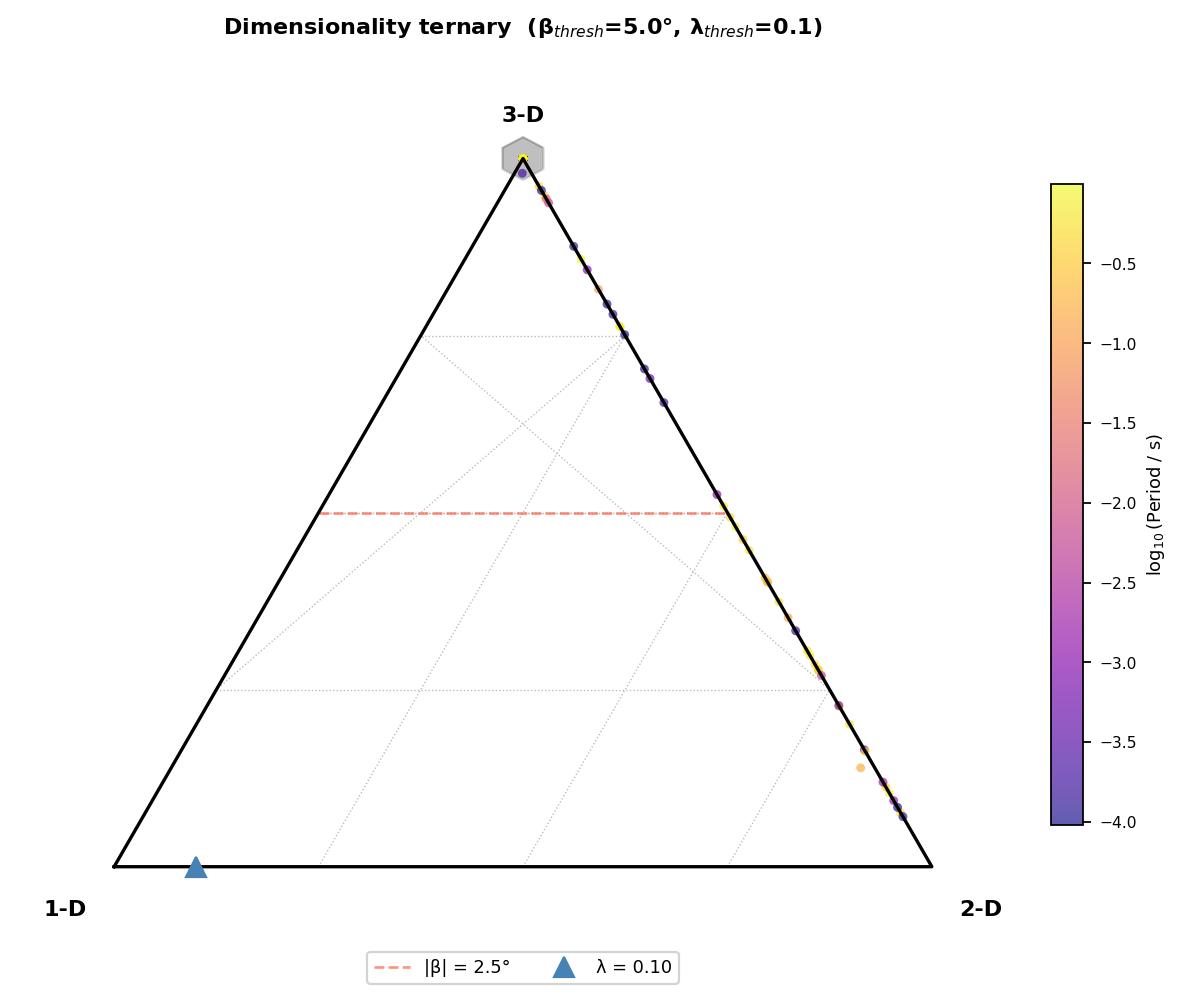
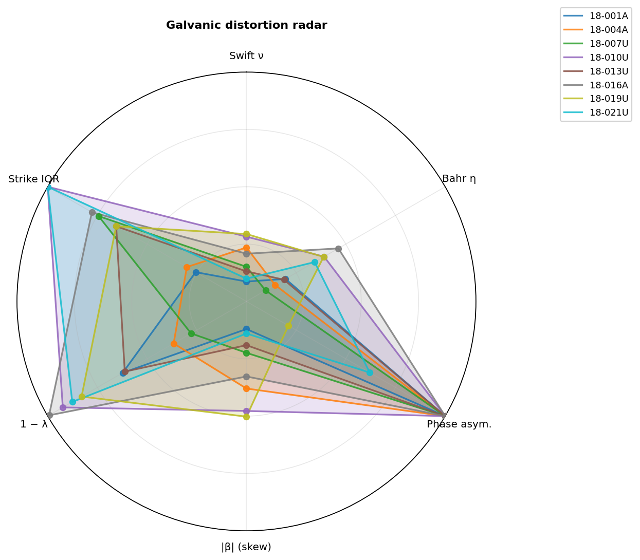
The ternary diagram maps each station-period cell into continuous 1-D, 2-D, and 3-D memberships, rather than forcing a hard class too early. The radar plot compares several distortion proxies per station, making it useful for choosing stations that need closer review before rotation, static-shift correction, or inversion.

11.25.6. Pseudosections And Survey Summaries

The survey-level functions are the most useful when preparing a processing report or deciding whether a line is ready for inversion.

>>> from pycsamt.emtools.advanced import (
...     plot_sensitivity_depth_section,
...     plot_apparent_anisotropy_section,
...     plot_dimensionality_depth_profile,
...     plot_z_invariants_section,
...     plot_survey_fingerprint,
...     plot_mt_composite_section,
...     plot_snr_section,
... )
>>> fig_depth = plot_sensitivity_depth_section(sites, component="xy")
>>> fig_aniso = plot_apparent_anisotropy_section(sites, show_pt_arrows=True)
>>> fig_dimdepth = plot_dimensionality_depth_profile(sites)
>>> fig_invariants = plot_z_invariants_section(sites)
>>> fig_fingerprint = plot_survey_fingerprint(sites)
>>> fig_composite = plot_mt_composite_section(sites, component="xy")
>>> fig_snr = plot_snr_section(sites, components=("xy",))

The sensitivity-depth, apparent-anisotropy, dimensionality-depth, and SNR sections are all single- or double-row station-period profiles with a similar wide aspect, so a two-by-two grid keeps them readable without wasted space:

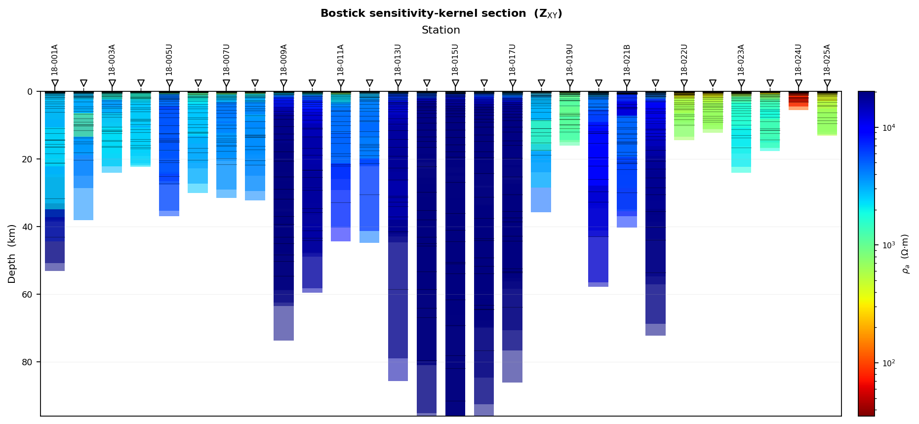
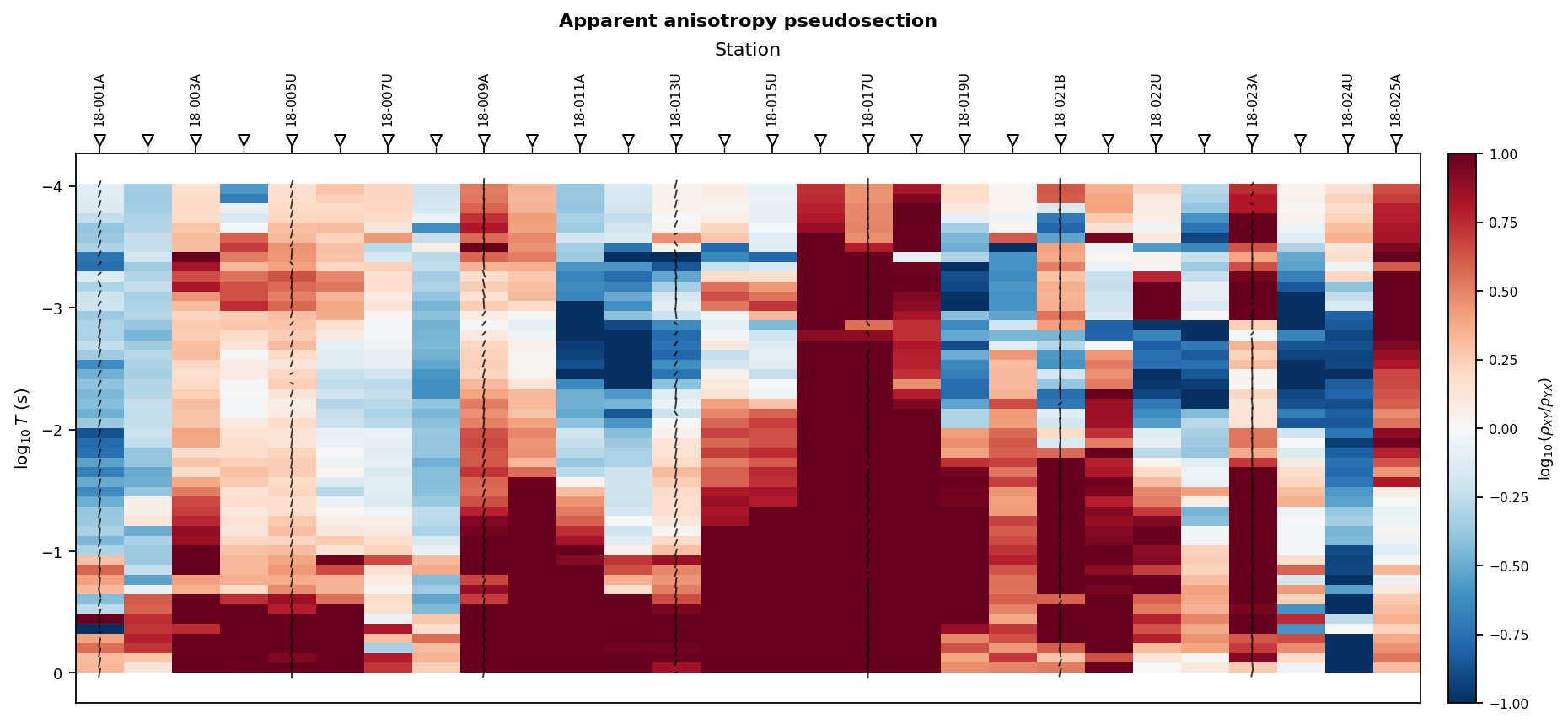
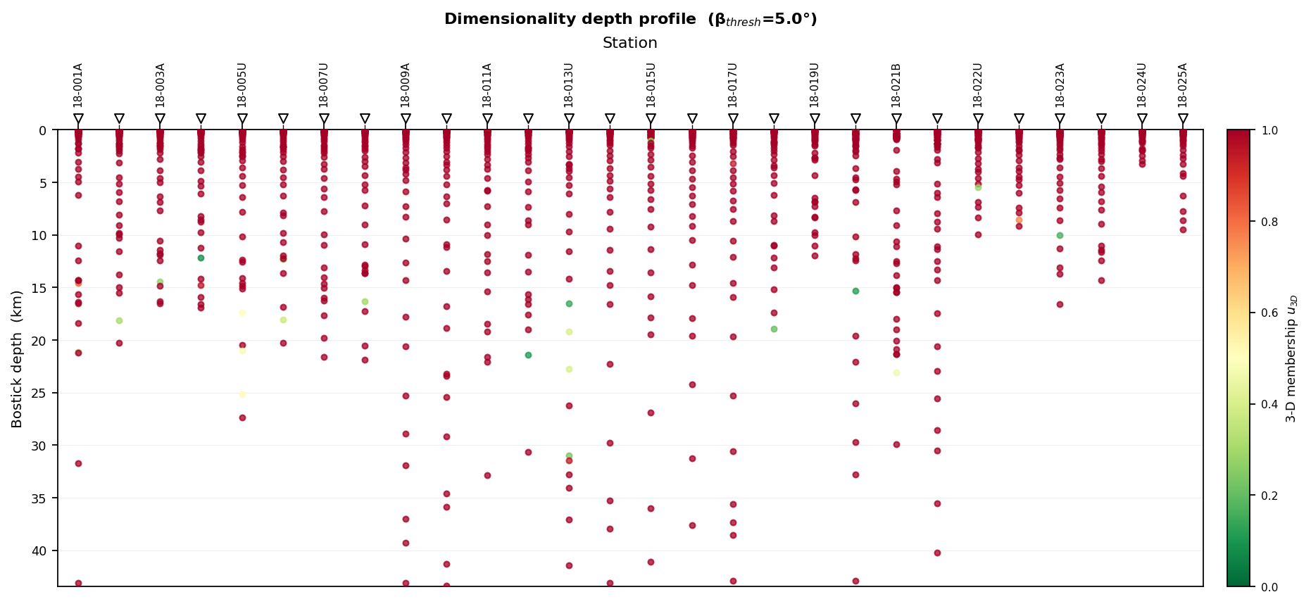
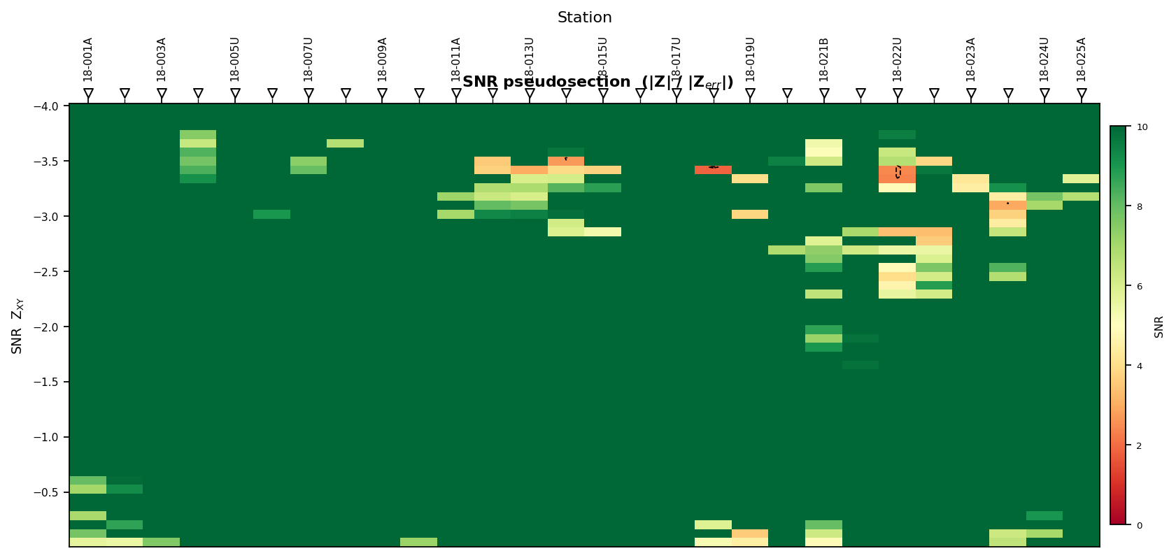
These four plots are profile-oriented: station along the horizontal axis, and period, pseudo-depth, or an anisotropy ratio along the vertical axis. Use them to find period bands with poor coverage, stations with local distortion, broad regions of anisotropy, or features that persist across independent diagnostics.

plot_z_invariants_section, plot_survey_fingerprint, and plot_mt_composite_section are denser, stacked-row dashboards – several metrics per figure – and stay easiest to read at full page width rather than compressed into a grid cell:

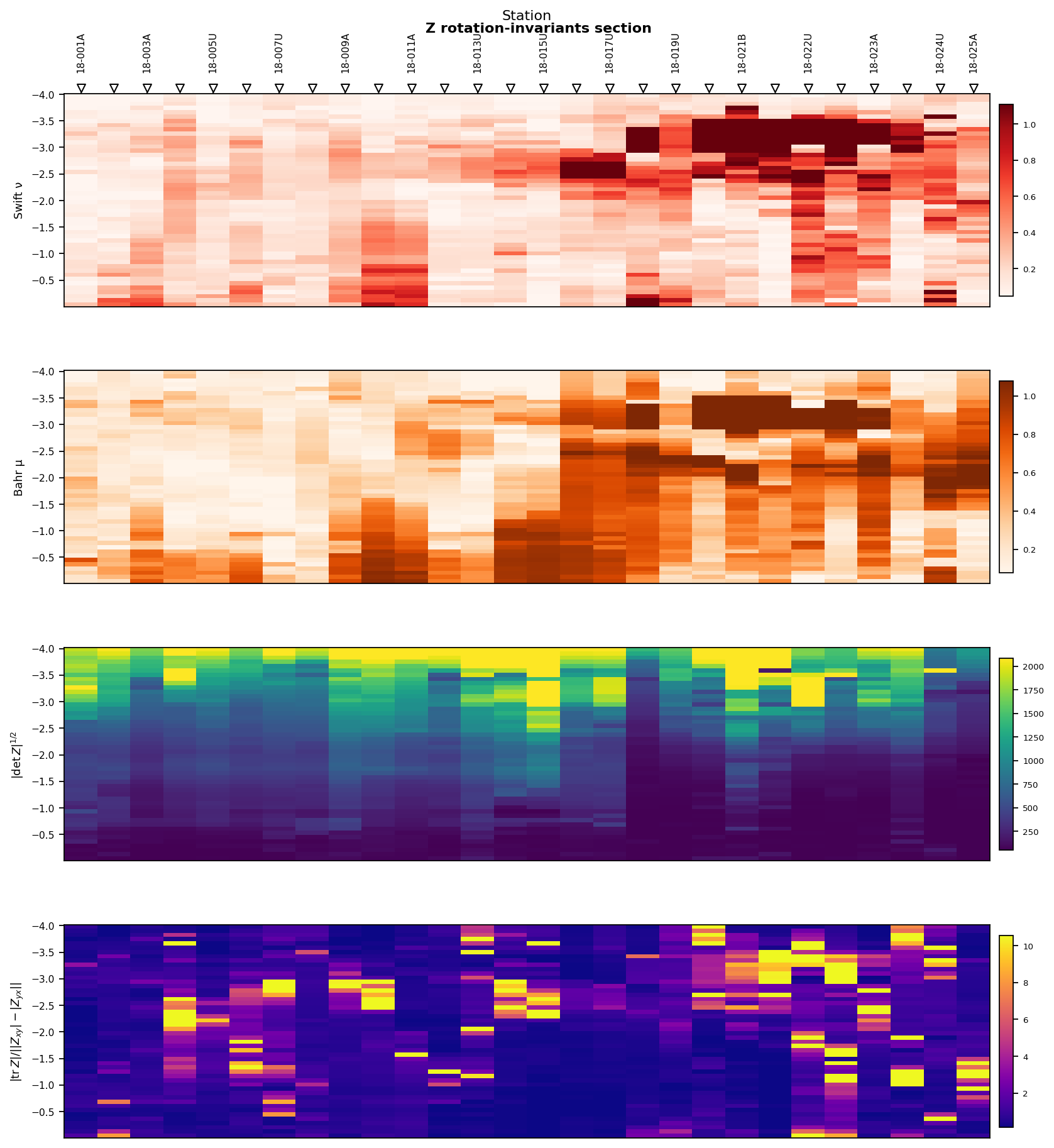
The four rotation-invariant panels (Swift nu, Bahr mu, determinant amplitude, and the trace-difference anisotropy proxy) are each less dependent on coordinate rotation than a single raw tensor component, which is why they are grouped together rather than shown as one number per station.

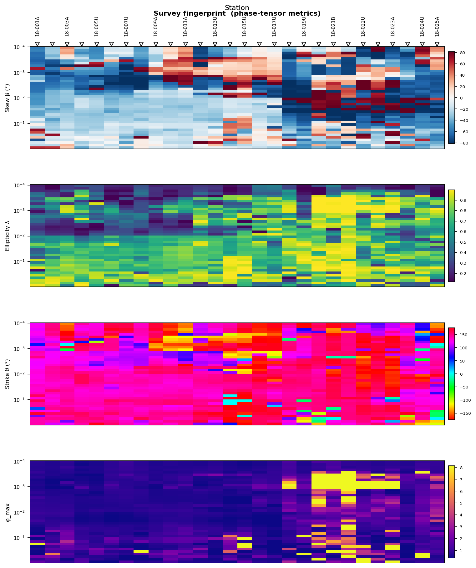
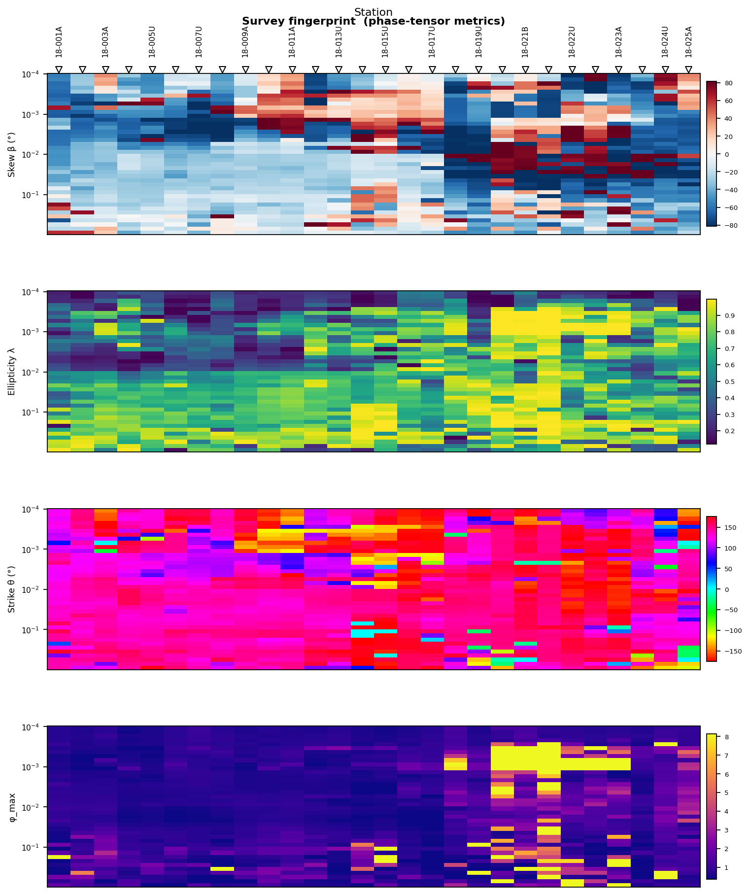
The survey fingerprint puts several phase-tensor metrics for the whole line on the same station-by-log-period grid, so a feature that aligns across skew, ellipticity, strike, and phase is harder to dismiss than one visible in only a single metric.

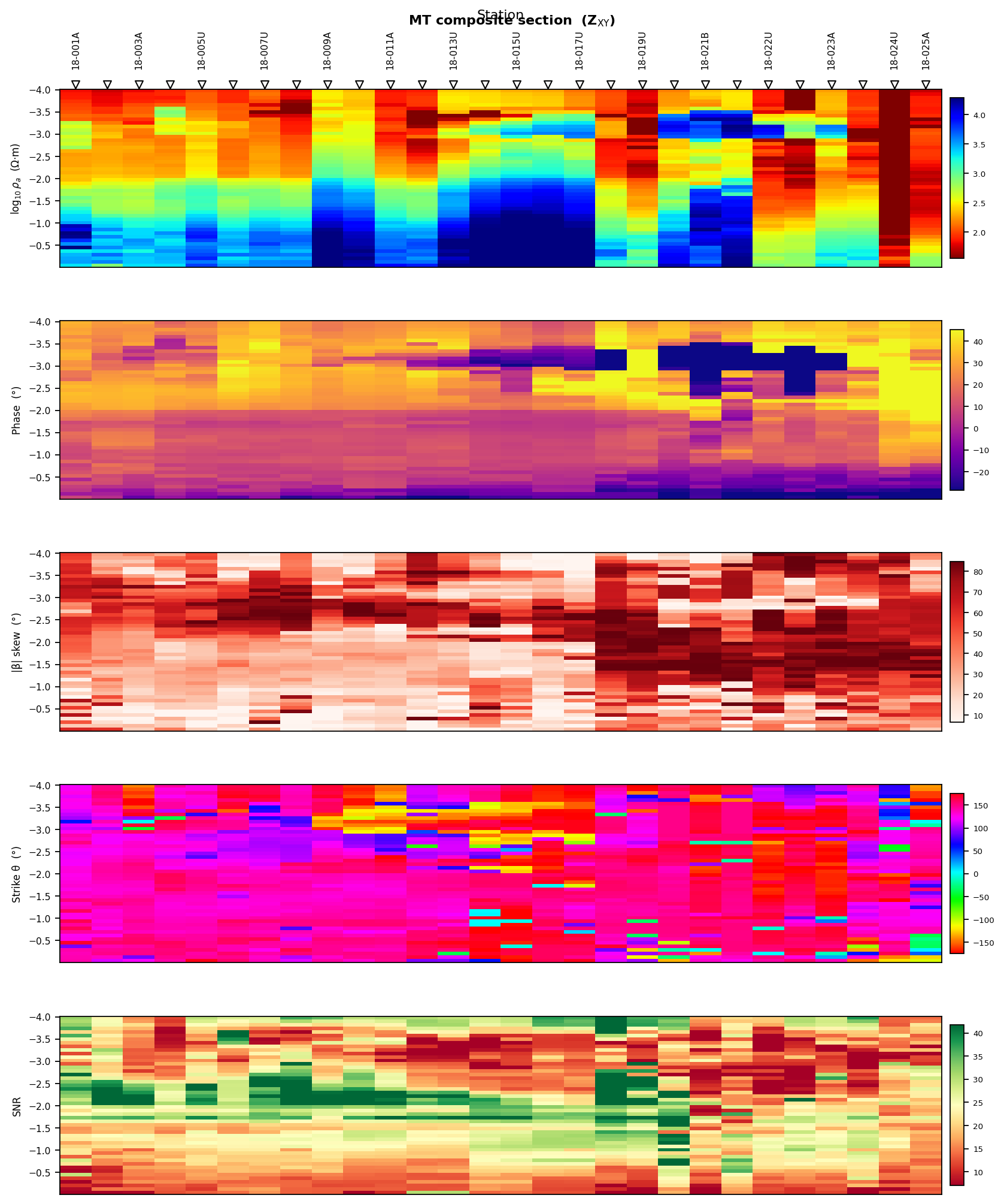
The composite section adds SNR to resistivity, phase, skew, and strike on that same grid, which is what lets you reject a tempting resistivity feature outright when it coincides with high skew or weak SNR at the same station and period.

11.25.7. Strike Stability And Coherence

Strike and coherence checks are useful late in QC, when the question is whether a chosen structural direction or station grouping is stable enough to justify downstream modelling decisions.

>>> from pycsamt.emtools.advanced import (
...     plot_strike_stability_bands,
...     plot_tf_coherence_network,
... )
>>> fig_strike = plot_strike_stability_bands(
...     sites,
...     methods=("pt", "swift", "bahr"),
...     period_range=(1e-3, 10.0),
... )
>>> fig_network = plot_tf_coherence_network(
...     sites,
...     component="xy",
...     threshold=0.90,
...     max_edges=100,
...     figsize=(7.5, 9.5),
... )

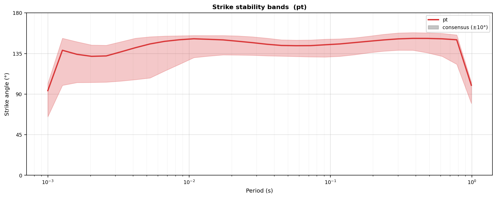
plot_strike_stability_bands compares strike estimates across methods and periods on a wide period axis:

plot_tf_coherence_network instead places stations at their real coordinates and connects station pairs whose transfer-function curves are highly correlated. L18PLT runs nearly north-south, so its station footprint is naturally tall and narrow rather than square – passing an explicit figsize keeps the map at a readable aspect instead of the very elongated canvas a default north-south layout would otherwise use:

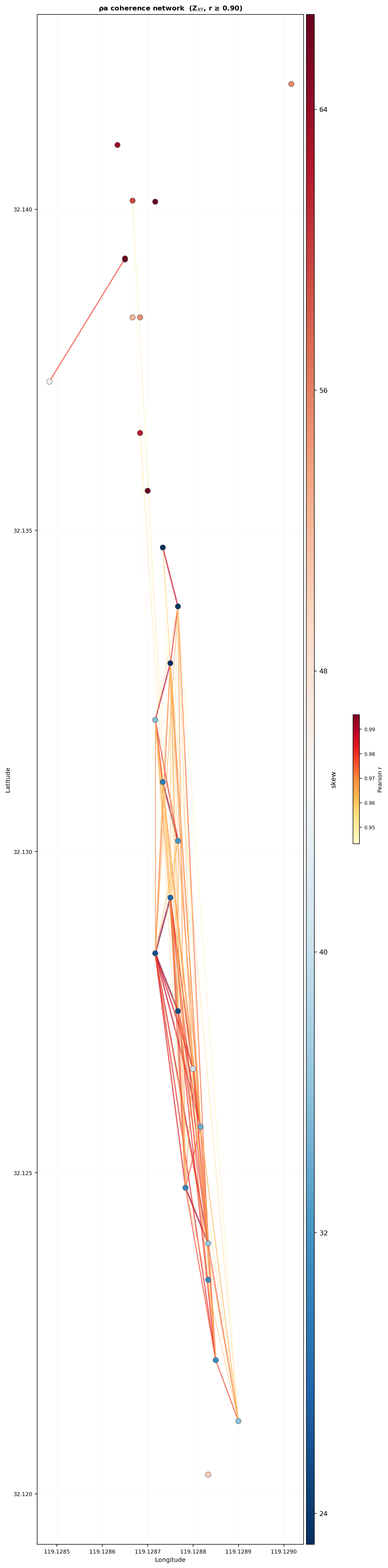
Connected stations have similar response curves in the selected band. Isolated stations may be outliers, locally distorted, poorly located, or geologically distinct.

11.25.8. Detailed Function Guide

This section is the dense practical guide for each function. It explains what the function computes, which parameters matter most, what code to write, and how to interpret the output.

11.25.8.1. Impedance Mohr Circles

plot_impedance_mohr_circles() diagnoses the rotational behaviour of the full impedance tensor at one station using an Impedance Mohr circle – useful groundwork before assuming that a station can be treated as 1-D or 2-D. For each selected period, the function rotates the 2 x 2 impedance tensor through n_theta angles with Z_rot = R @ Z @ R.T, then traces two selected tensor components as closed curves in separate real and imaginary panels. For component pair \(a,b\), the real-panel trajectory is

\[\theta \mapsto \left(\Re Z_{\theta,a}, \Re Z_{\theta,b}\right),\]

and the imaginary-panel trajectory is

\[\theta \mapsto \left(\Im Z_{\theta,a}, \Im Z_{\theta,b}\right).\]

Each selected period therefore gives one closed curve. Period color coding shows whether the rotational behaviour is shallow-only, deep-only, or persistent across the sounding.

Key parameters

station selects the station; periods gives exact target periods; n_periods chooses log-spaced periods automatically; components chooses the tensor entries plotted against each other.

>>> from pycsamt.emtools.advanced import plot_impedance_mohr_circles
>>> fig = plot_impedance_mohr_circles(
...     sites,
...     station="18-001A",
...     n_periods=8,
...     n_theta=360,
...     components=("xx", "xy"),
...     recursive=False,
... )
>>> fig.savefig(out / "mohr_circles_18-001A.png", dpi=200)

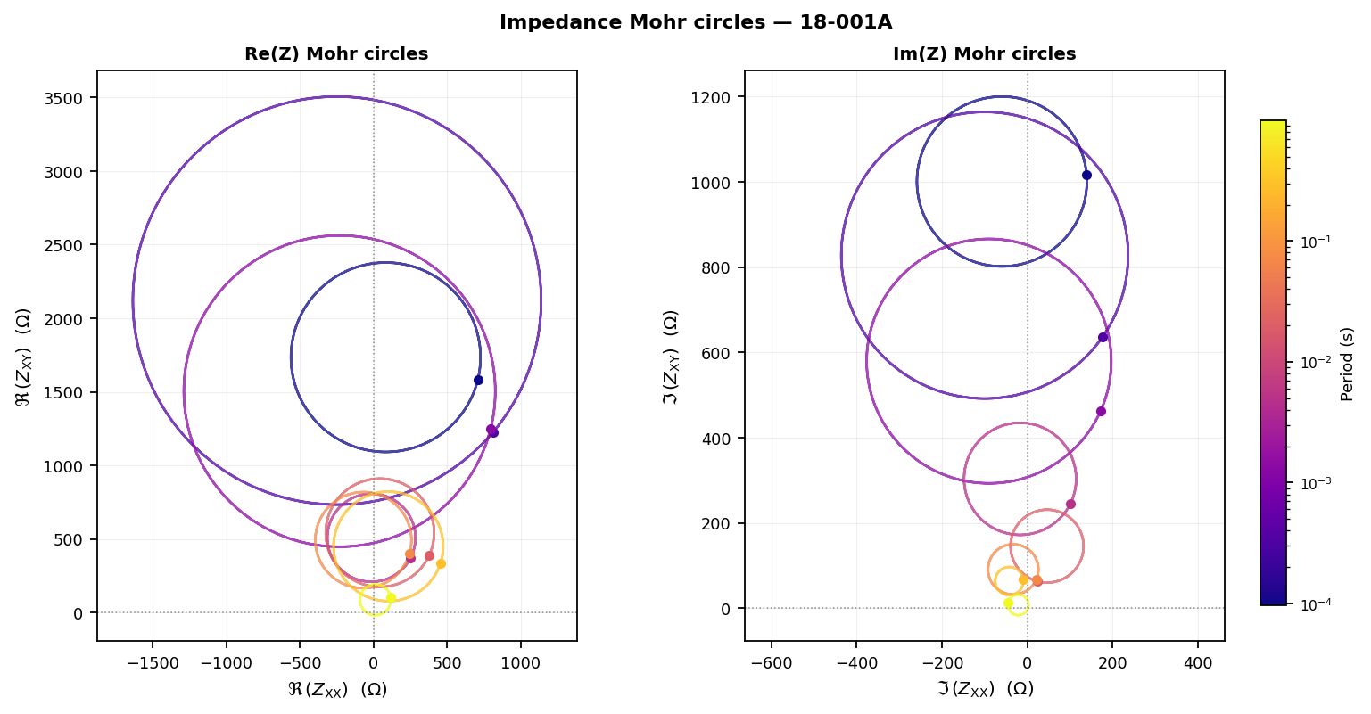
A 1-D response collapses toward points. A 2-D response produces circles that pass through the origin. A 3-D response produces circles offset from the origin. Strongly period-dependent offsets are a warning that simple dimensional assumptions should be checked with phase tensor and skew tools.

11.25.8.2. Argand Trajectories

plot_zt_argand() shows impedance components directly in the complex plane, using period as the trajectory coordinate – an Argand diagram of the tensor. It extracts each requested component, sorts samples by period, plots Re(Z_ij) against Im(Z_ij), color-codes by period, and adds arrows in the direction of increasing period. For component \(Z_{ij}\), the plotted trajectory is

\[\gamma_{ij}(T) = \left( \Re Z_{ij}(T), \Im Z_{ij}(T) \right).\]

With normalize=True, the component is divided by a robust amplitude scale before plotting, so the diagram emphasizes trajectory shape rather than absolute impedance magnitude.

Key parameters

components controls the tensor entries; period_range isolates a band; normalize=True removes amplitude and emphasizes trajectory shape.

>>> from pycsamt.emtools.advanced import plot_zt_argand
>>> fig = plot_zt_argand(
...     sites,
...     station="18-001A",
...     components=("xy", "yx"),
...     period_range=(1e-3, 10.0),
...     normalize=False,
...     recursive=False,
... )
>>> fig.savefig(out / "argand_18-001A.png", dpi=200)

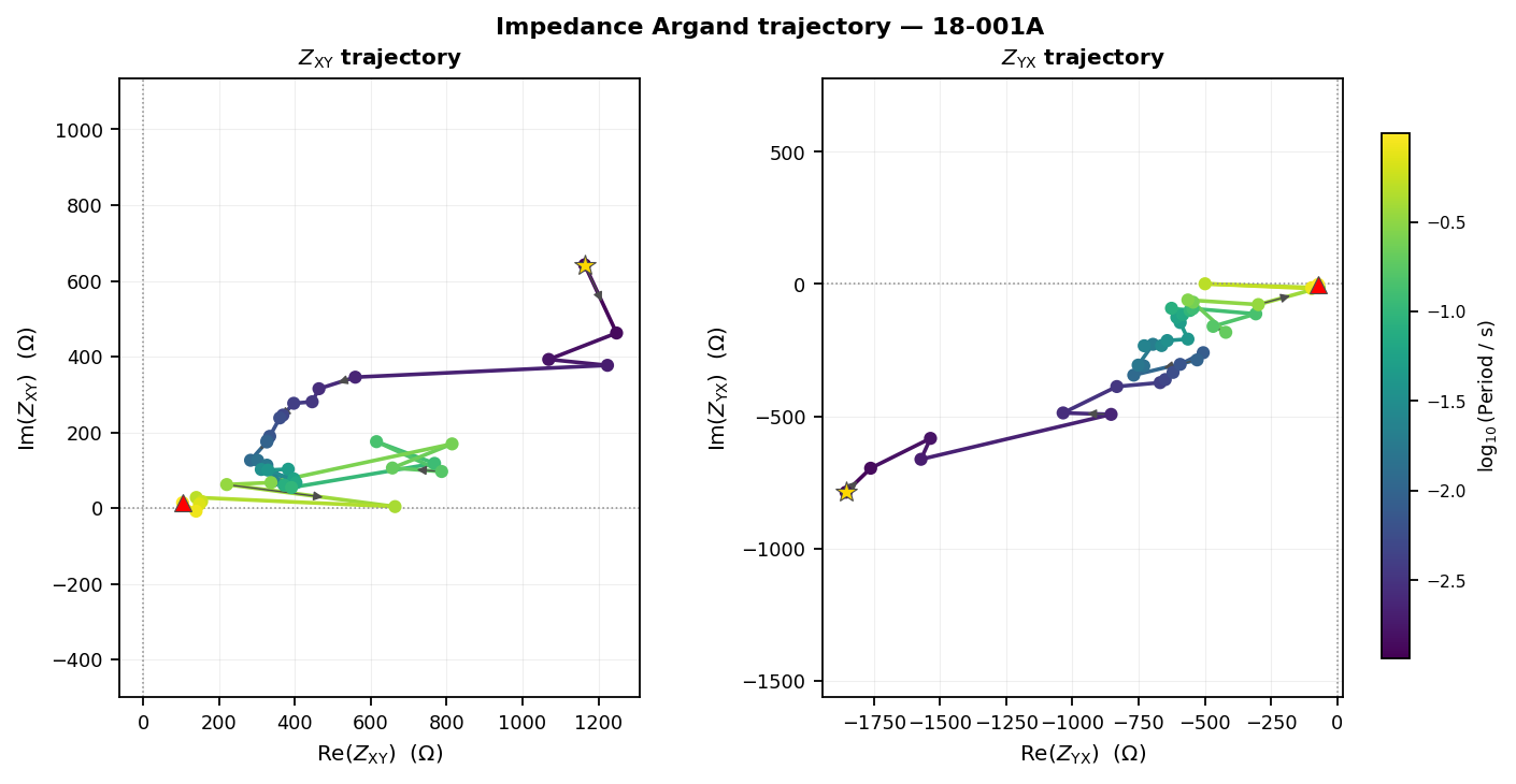
Smooth, simple trajectories are easier to reconcile with layered structure. Loops, sharp bends, or large differences between Zxy and Zyx indicate lateral complexity, distortion, or component-specific problems.

11.25.8.3. Bode Rho-Phase Consistency

plot_rho_phase_bode() tests Bode consistency – whether observed phase agrees with the local slope of apparent resistivity under a minimum-phase assumption. It computes an approximate Bode phase,

\[\phi_{Bode}(T) \approx 45^\circ \left(1 + {d\log\rho_a \over d\log T}\right),\]

and compares it to the observed phase. In the code, the derivative is estimated directly on the sampled curve \(\log_{10}\rho_a\) versus \(\log_{10}T\):

\[s(T) = {d\log_{10}\rho_a \over d\log_{10}T}, \qquad \phi_\mathrm{Bode}(T) = 45^\circ(1+s(T)).\]

The shaded area in the plot is the discrepancy between \(\phi_\mathrm{obs}\) and \(\phi_\mathrm{Bode}\).

Key parameters

component chooses "xy" or "yx"; smooth_window applies a centered moving average before the derivative is estimated.

>>> from pycsamt.emtools.advanced import plot_rho_phase_bode
>>> fig = plot_rho_phase_bode(
...     sites,
...     station="18-001A",
...     component="xy",
...     smooth_window=1,
...     recursive=False,
... )
>>> fig.savefig(out / "bode_consistency_18-001A.png", dpi=200)

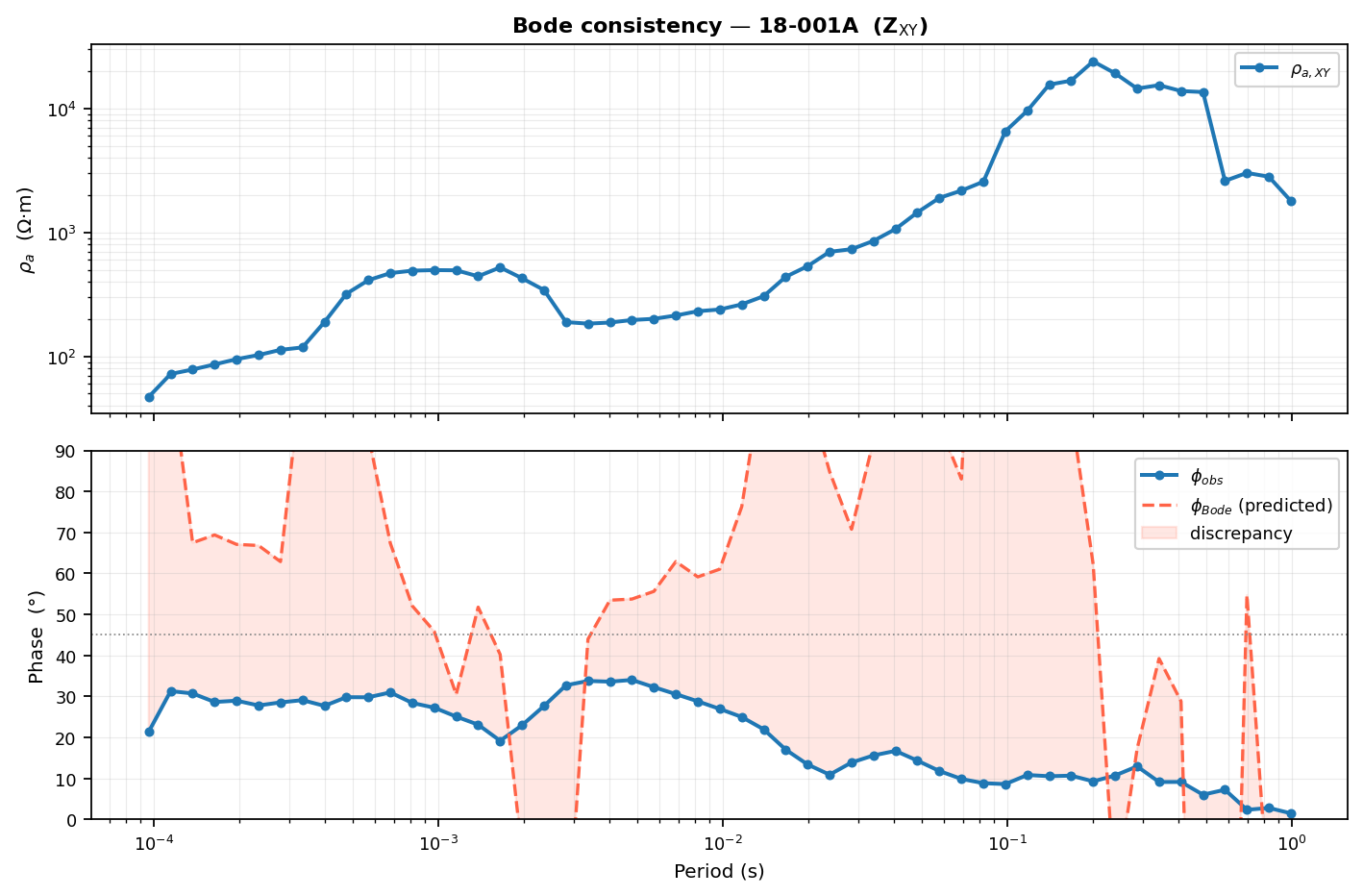
If observed and predicted phase track one another, the response is more consistent with minimum-phase behaviour. Persistent separation can indicate galvanic distortion, source effects, or a response that is too complex for a simple layered model.

11.25.8.4. Apparent-Resistivity Polar Diagram

plot_apparent_resistivity_polar() inspects directional dependence of apparent resistivity as the impedance tensor is rotated. For selected periods, the tensor is rotated through 360 degrees and rho_a_xy(theta) is computed at each angle, so each period becomes one polar petal with radius

\[r_\rho(\theta, f) = \rho_{a,xy}(\theta, f) = {0.2 \over f} |Z_{\theta,xy}(f)|^2.\]

With normalize=True, each period is instead scaled by its own maximum,

\[\tilde{r}_\rho(\theta, f) = {r_\rho(\theta, f) \over \max_\theta r_\rho(\theta, f)},\]

which lets the user compare directional shape across periods even when absolute apparent resistivity changes strongly.

Key parameters

n_periods controls the number of petals; normalize=True emphasizes petal shape rather than amplitude; period_range restricts periods.

>>> from pycsamt.emtools.advanced import plot_apparent_resistivity_polar
>>> fig = plot_apparent_resistivity_polar(
...     sites,
...     station="18-001A",
...     n_periods=8,
...     normalize=True,
...     recursive=False,
... )
>>> fig.savefig(out / "rho_polar_18-001A.png", dpi=200)

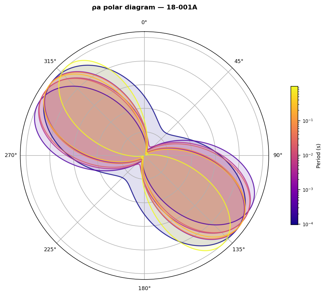
Circular petals indicate weak directional dependence. Elongated petals indicate anisotropy or 2-D behaviour. Petals whose orientation rotates with period suggest depth-dependent structure or distortion.

11.25.8.5. Phase-Tensor Period Clock

plot_pt_period_clock() compresses phase tensor strike and ellipticity across period into one radial figure. It builds the phase-tensor table, chooses log-spaced period rings, and draws an ellipse on each ring – if station is omitted, it uses survey-median values instead. The phase tensor itself is

\[\boldsymbol{\Phi}(f) = \Re(\mathbf{Z}(f))^{-1} \Im(\mathbf{Z}(f)),\]

and each ring uses the median phase-tensor strike \(\theta_\Phi\) and ellipticity \(e_\Phi\) in that period neighborhood: the ellipse is rotated by \(\theta_\Phi\), and its minor axis is shortened as ellipticity grows.

Key parameters

station switches between station-specific and survey-median mode; n_rings controls period sampling; period_range clips the depth window.

>>> from pycsamt.emtools.advanced import plot_pt_period_clock
>>> fig = plot_pt_period_clock(
...     sites,
...     station="18-001A",
...     n_rings=7,
...     period_range=(1e-3, 10.0),
...     recursive=False,
... )
>>> fig.savefig(out / "pt_clock_18-001A.png", dpi=200)

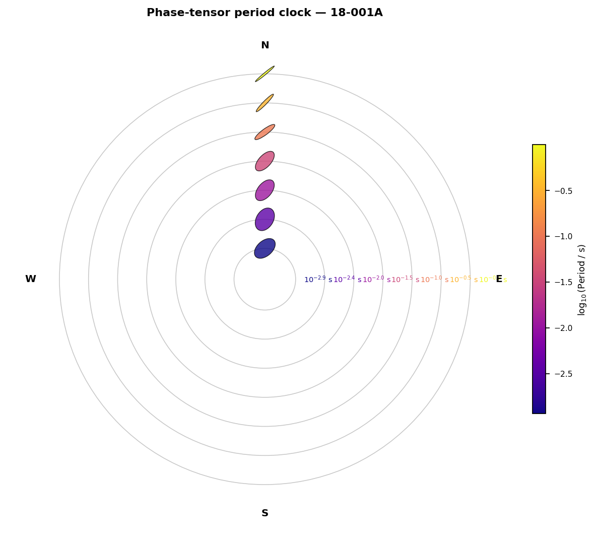
Stable ellipse orientation suggests a persistent structural direction. Rotation with period suggests depth-dependent strike or 3-D structure. Strong elongation indicates phase-tensor anisotropy.

11.25.8.6. Dimensionality Ternary

plot_dimensionality_ternary() displays station-period cells on a ternary diagram of continuous 1-D, 2-D, and 3-D memberships instead of forcing a hard class too early. It derives phase-tensor skew and ellipticity from pycsamt.emtools.tensor.build_phase_tensor_table(), where skew controls 3-D membership while ellipticity helps separate 1-D and 2-D behaviour when skew is low. The soft memberships are

\[u_{3D} = \operatorname{clip} \left({|\beta| \over \beta_\mathrm{th}},0,1\right),\]

\[u_{1D} = (1-u_{3D}) \operatorname{clip} \left(1-{e \over e_\mathrm{th}},0,1\right), \qquad u_{2D}=1-u_{1D}-u_{3D},\]

where \(\beta\) is phase-tensor skew, \(e\) is ellipticity, and the thresholds are beta_thresh and ellipt_thresh. The plotted ternary point is the barycentric coordinate \((u_{1D},u_{2D},u_{3D})\).

Key parameters

beta_thresh controls how quickly skew maps to 3-D membership; ellipt_thresh controls ellipticity sensitivity; period_range selects the band.

>>> from pycsamt.emtools.advanced import plot_dimensionality_ternary
>>> fig = plot_dimensionality_ternary(
...     sites,
...     beta_thresh=5.0,
...     ellipt_thresh=0.1,
...     period_range=(1e-3, 10.0),
...     recursive=False,
... )
>>> fig.savefig(out / "dimensionality_ternary.png", dpi=200)

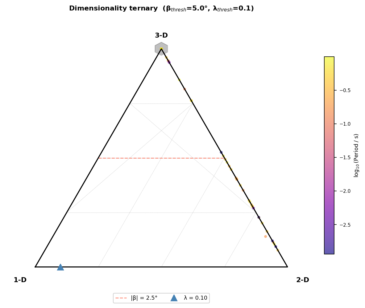
A cloud near the 1-D corner supports simple layered assumptions. A cloud along the 2-D edge suggests strike analysis may be meaningful. A cloud near the 3-D corner warns against simple 1-D or 2-D inversion assumptions.

11.25.8.7. Distortion Radar

plot_distortion_radar() compares several distortion proxies at selected stations. Each station is summarized by multiple normalized proxies – Swift-style behaviour, Bahr-style behaviour, phase asymmetry, absolute skew, ellipticity-related behaviour, and strike instability – and becomes one polygon. Two of the radar axes are

\[\nu = {|Z_{xx}+Z_{yy}| \over |Z_{xy}-Z_{yx}|+\varepsilon}, \qquad \eta = {|Z_{xy}+Z_{yx}| \over |Z_{xy}-Z_{yx}|+\varepsilon},\]

converted to bounded scores with \(s=\nu/(1+\nu)\) or \(s=\eta/(1+\eta)\). Phase asymmetry is summarized from \(|\phi_{xy}+\phi_{yx}-180^\circ|/90^\circ\), while strike instability comes from the interquartile range of phase-tensor strike angles in the selected band.

Key parameters

stations selects named stations; max_stations limits automatic selection; period_range controls the summary band.

>>> from pycsamt.emtools.advanced import plot_distortion_radar
>>> fig = plot_distortion_radar(
...     sites,
...     max_stations=8,
...     period_range=(1e-3, 10.0),
...     recursive=False,
... )
>>> fig.savefig(out / "distortion_radar.png", dpi=200)

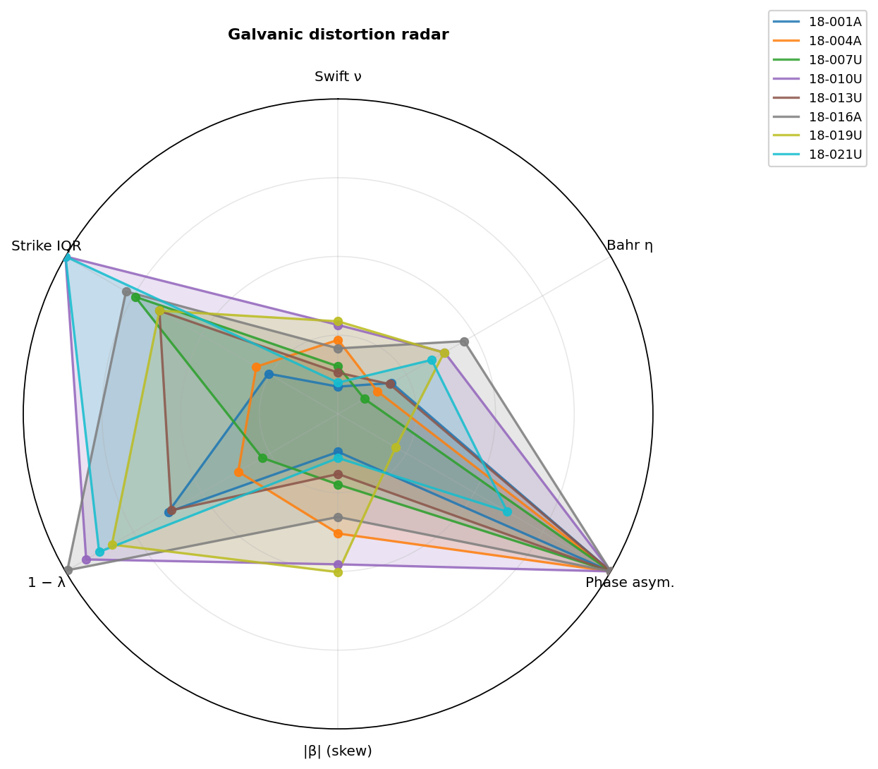
Compact polygons suggest lower distortion. Large polygons or stations with very different shapes deserve closer station-level review before inversion.

11.25.8.8. Sensitivity-Depth Section

plot_sensitivity_depth_section() shows where each station-period datum is sensitive in pseudo-depth space. For each valid apparent-resistivity datum, it computes Bostick depth,

\[d_B = \sqrt{\rho_a / (\mu_0 2 \pi f)},\]

then draws a vertical bar centered at that depth: color encodes rho_a, and bar height approximates the sensitivity window from the local slope

\[q(T) = {d\log_{10}\rho_a \over d\log_{10}T}.\]

Large changes in this slope imply a broader or less stable pseudo-depth contribution, so read the section as sensitivity coverage rather than as a resolved layer boundary.

Key parameters

component selects "xy" or "yx"; depth_unit selects "km" or "m"; depth_max clips the view; rho_lim fixes color limits across surveys.

>>> from pycsamt.emtools.advanced import plot_sensitivity_depth_section
>>> fig = plot_sensitivity_depth_section(
...     sites,
...     component="xy",
...     depth_unit="km",
...     depth_max=5.0,
...     recursive=False,
... )
>>> fig.savefig(out / "sensitivity_depth_xy.png", dpi=200)

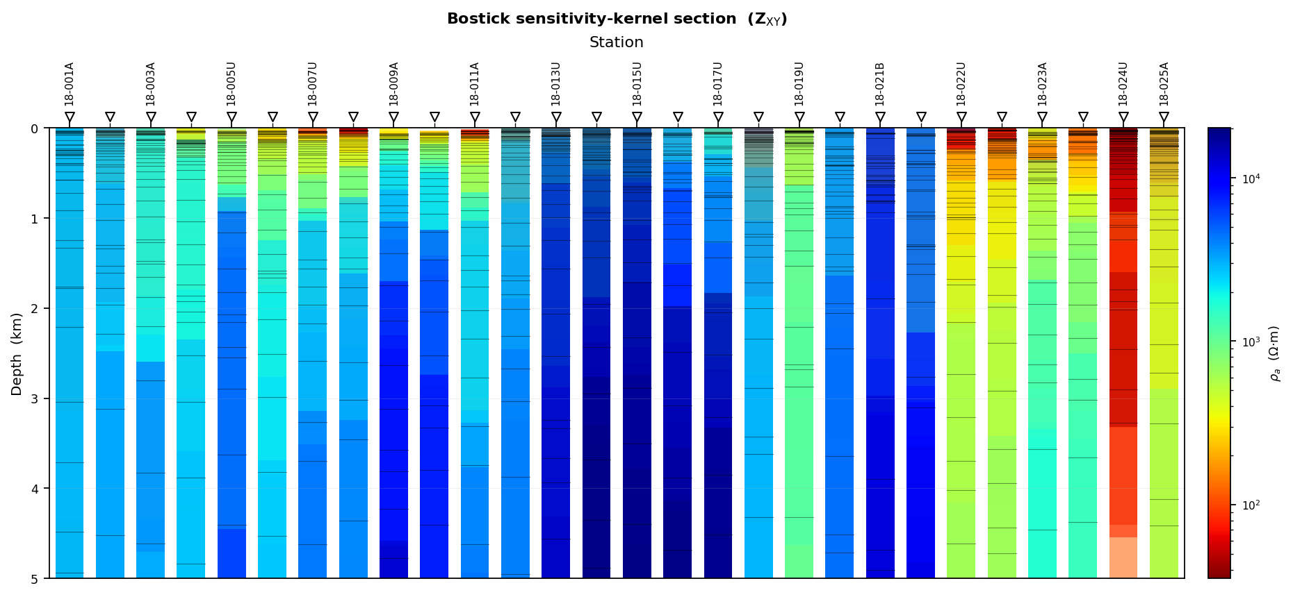
Dense overlapping bars indicate stronger depth coverage. Gaps indicate weak coverage. Very broad windows mean lower vertical resolution.

11.25.8.9. Apparent-Anisotropy Section

plot_apparent_anisotropy_section() compares the two off-diagonal apparent-resistivity modes along the profile as a proxy for anisotropy. The plotted value is log10(rho_xy / rho_yx), so warm cells mean rho_xy is larger and cool cells mean rho_yx is larger. Formally, the displayed proxy is

\[A_\rho = \log_{10} \left({\rho_{xy}\over\rho_{yx}}\right),\]

so \(A_\rho=0\) means the two off-diagonal modes agree, \(A_\rho=1\) means \(\rho_{xy}\) is ten times \(\rho_{yx}\), and \(A_\rho=-1\) means the reverse.

Key parameters

show_pt_arrows=True overlays phase-tensor principal-axis directions; arrow_every thins the arrows; vmax sets symmetric color limits.

>>> from pycsamt.emtools.advanced import plot_apparent_anisotropy_section
>>> fig = plot_apparent_anisotropy_section(
...     sites,
...     period_range=(1e-3, 10.0),
...     show_pt_arrows=True,
...     arrow_every=3,
...     vmax=1.0,
...     recursive=False,
... )
>>> fig.savefig(out / "apparent_anisotropy.png", dpi=200)

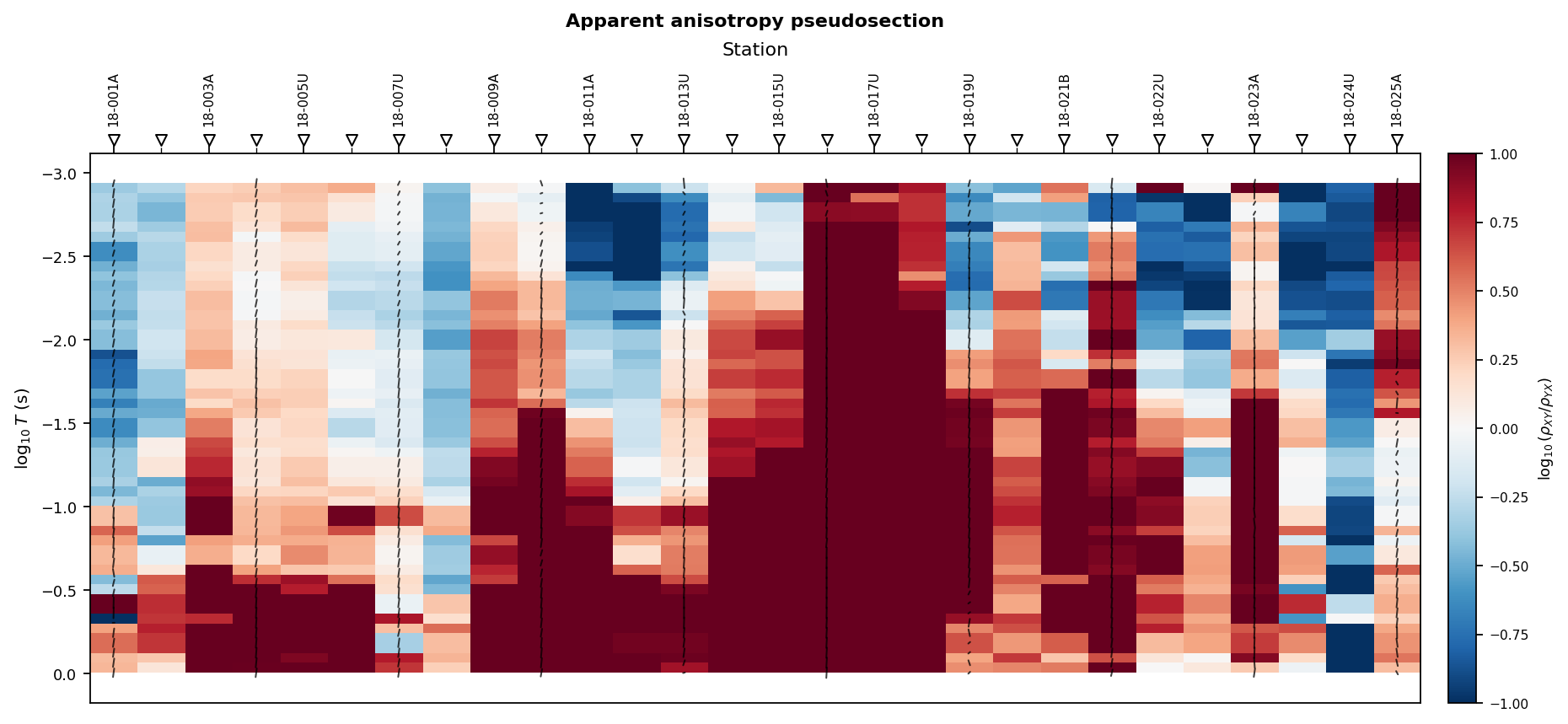
Coherent warm or cool bands can indicate profile-scale anisotropy or structural directionality. Isolated station anomalies often point to local distortion or station problems.

11.25.8.10. Dimensionality-Depth Profile

plot_dimensionality_depth_profile() places dimensionality membership into pseudo-depth space. Phase-tensor skew and ellipticity are converted into 3-D membership, and each period sample is placed at Bostick depth using the selected impedance component. The color value is

\[u_{3D} = \operatorname{clip} \left({|\beta| \over \beta_\mathrm{th}},0,1\right),\]

the same 3-D membership used by the ternary plot. The vertical coordinate is pseudo-depth, so clusters of high \(u_{3D}\) mark depth intervals where simple dimensional assumptions are least reliable.

Key parameters

component controls the apparent resistivity used for depth; beta_thresh and ellipt_thresh control membership sensitivity; depth_max clips the displayed pseudo-depth range.

>>> from pycsamt.emtools.advanced import plot_dimensionality_depth_profile
>>> fig = plot_dimensionality_depth_profile(
...     sites,
...     component="xy",
...     beta_thresh=5.0,
...     ellipt_thresh=0.1,
...     depth_max=5.0,
...     recursive=False,
... )
>>> fig.savefig(out / "dimensionality_depth.png", dpi=200)

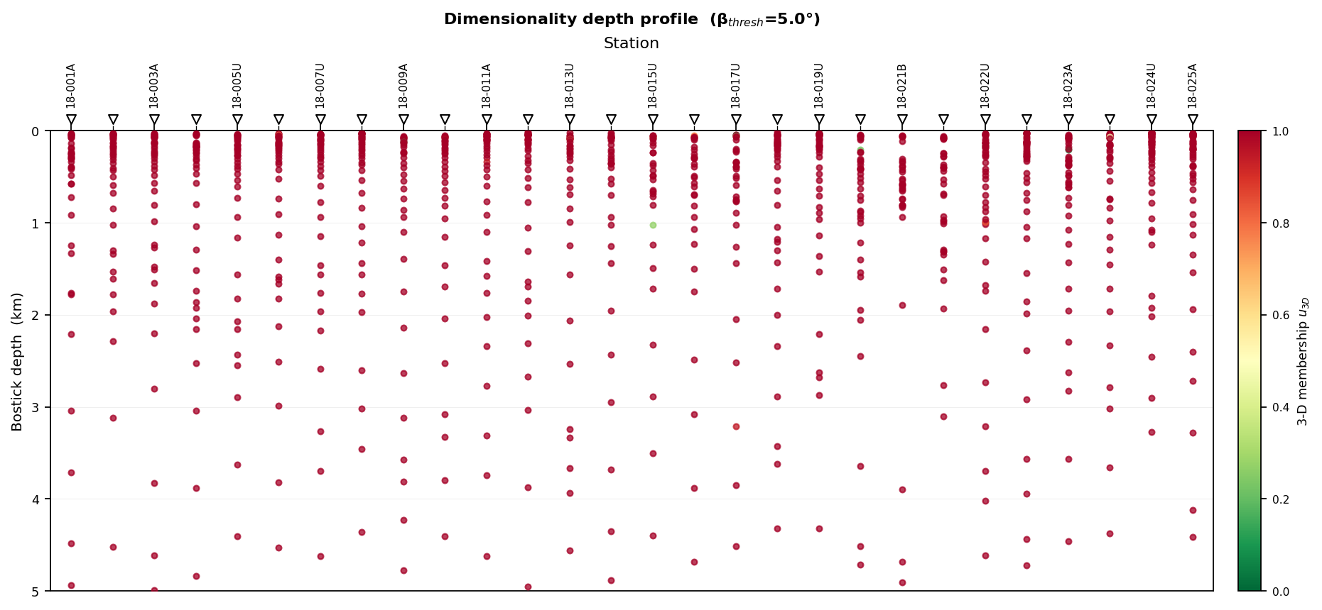
High 3-D membership at depth warns against simple inversion assumptions in that interval. Shallow isolated anomalies should be compared with static-shift and QC outputs.

11.25.8.11. Z Rotation-Invariants Section

plot_z_invariants_section() inspects impedance quantities that are less dependent on coordinate rotation than raw tensor components. Its four panels are Swift nu, Bahr mu, sqrt(abs(det Z)), and an anisotropy proxy based on trace magnitude relative to the difference between off-diagonal magnitudes. The determinant panel uses

\[|\det\mathbf{Z}|^{1/2} = |Z_{xx}Z_{yy}-Z_{xy}Z_{yx}|^{1/2},\]

and the trace-difference proxy uses

\[\chi = {|Z_{xx}+Z_{yy}| \over ||Z_{xy}|-|Z_{yx}||+\varepsilon}.\]

These panels are more robust than single raw tensor components, but high values should still be treated as prompts for closer review rather than standalone geological labels.

Key parameters

period_range isolates a band; station_order preserves profile order; axes embeds the four panels in a custom figure.

>>> from pycsamt.emtools.advanced import plot_z_invariants_section
>>> fig = plot_z_invariants_section(
...     sites,
...     period_range=(1e-3, 10.0),
...     recursive=False,
... )
>>> len(fig.axes)
4
>>> fig.savefig(out / "z_invariants.png", dpi=200)

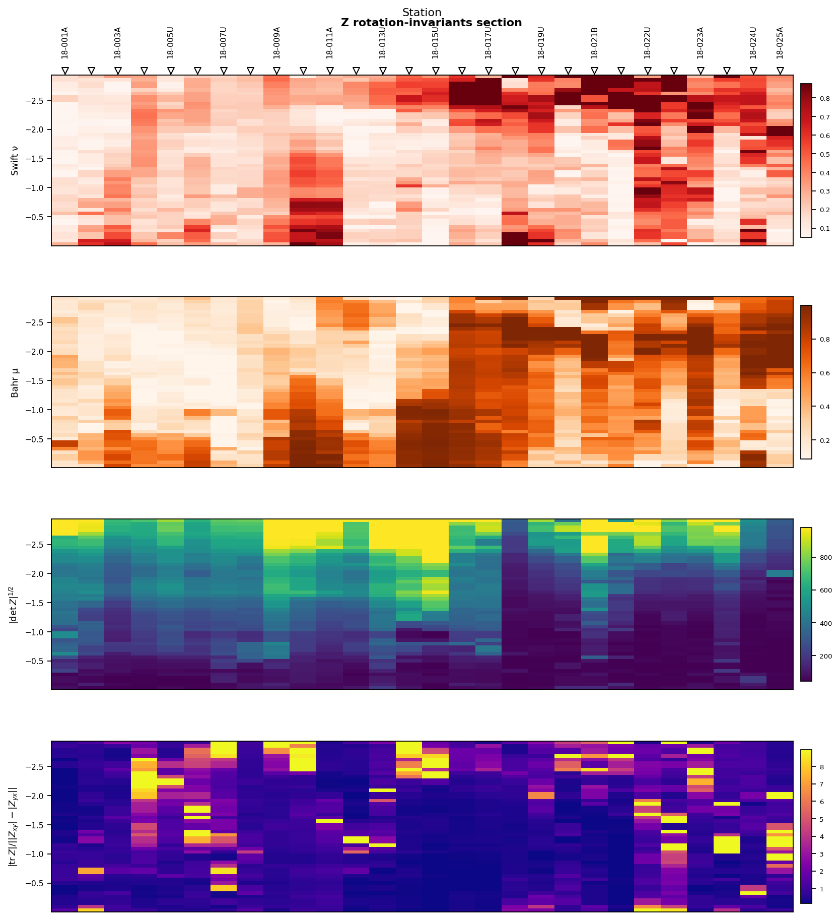
Low Swift and Bahr values are more compatible with 2-D assumptions. High persistent values warn of distortion or 3-D structure. The determinant panel gives a useful mode-independent amplitude proxy.

11.25.8.12. Survey Fingerprint

plot_survey_fingerprint() puts multiple phase-tensor metrics for the entire survey on one compact page. Each panel is a station-by-log-period image; default quantities include skew, ellipticity, strike angle, and maximum phase, with minimum phase and absolute skew available as options. The fingerprint is useful precisely because all panels share the same grid \((s,\log_{10}T)\) – a feature visible in only one metric may be metric-specific, whereas a feature that aligns across skew, ellipticity, strike, and phase is harder to dismiss.

Key parameters

quantities selects metrics; cell_aspect changes cell proportions; station_order fixes station sequence.

>>> from pycsamt.emtools.advanced import plot_survey_fingerprint
>>> fig = plot_survey_fingerprint(
...     sites,
...     quantities=["skew", "ellipt", "theta", "s1", "beta"],
...     period_range=(1e-3, 10.0),
...     recursive=False,
... )
>>> fig.savefig(out / "survey_fingerprint.png", dpi=200)

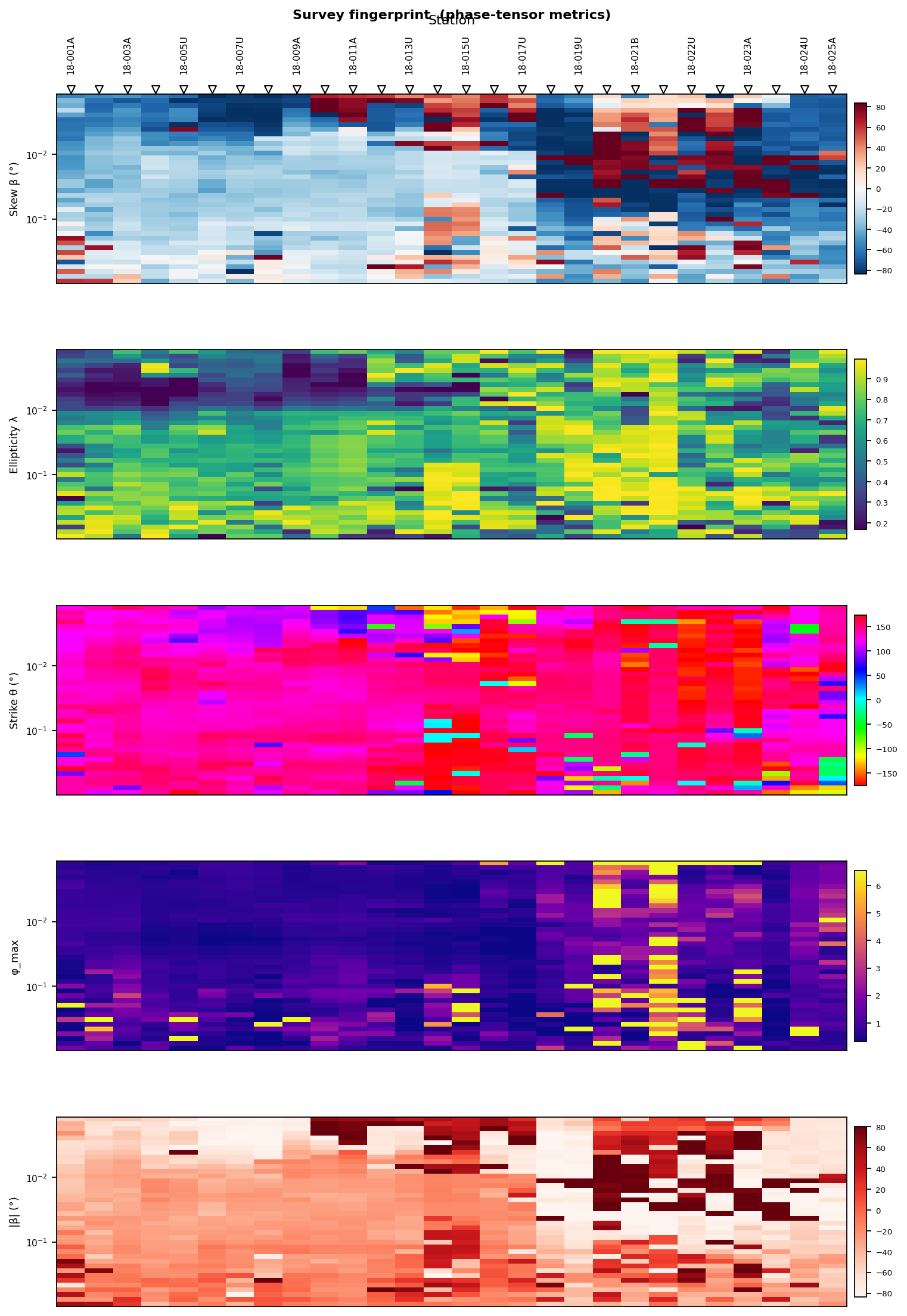
Use this as a review dashboard. Look for bands that align across metrics: high skew with high ellipticity, abrupt strike changes, or stations that stand apart from their neighbors.

11.25.8.13. MT Composite Section

plot_mt_composite_section() aligns several common MT diagnostics on a shared station-period grid: apparent resistivity (in log10 space), phase, absolute skew, strike, and SNR. The default rows combine

\[\log_{10}\rho_a,\quad \phi,\quad |\beta|,\quad \theta_\Phi,\quad \mathrm{SNR}\]

on that same station-period grid, which lets you reject a tempting resistivity feature outright if it occurs exactly where skew is high or SNR is weak.

Key parameters

component chooses "xy" or "yx" for rho, phase, and SNR; quantities controls rows.

>>> from pycsamt.emtools.advanced import plot_mt_composite_section
>>> fig = plot_mt_composite_section(
...     sites,
...     component="xy",
...     quantities=["rho", "phase", "skew", "theta", "snr"],
...     period_range=(1e-3, 10.0),
...     recursive=False,
... )
>>> fig.savefig(out / "mt_composite_xy.png", dpi=200)

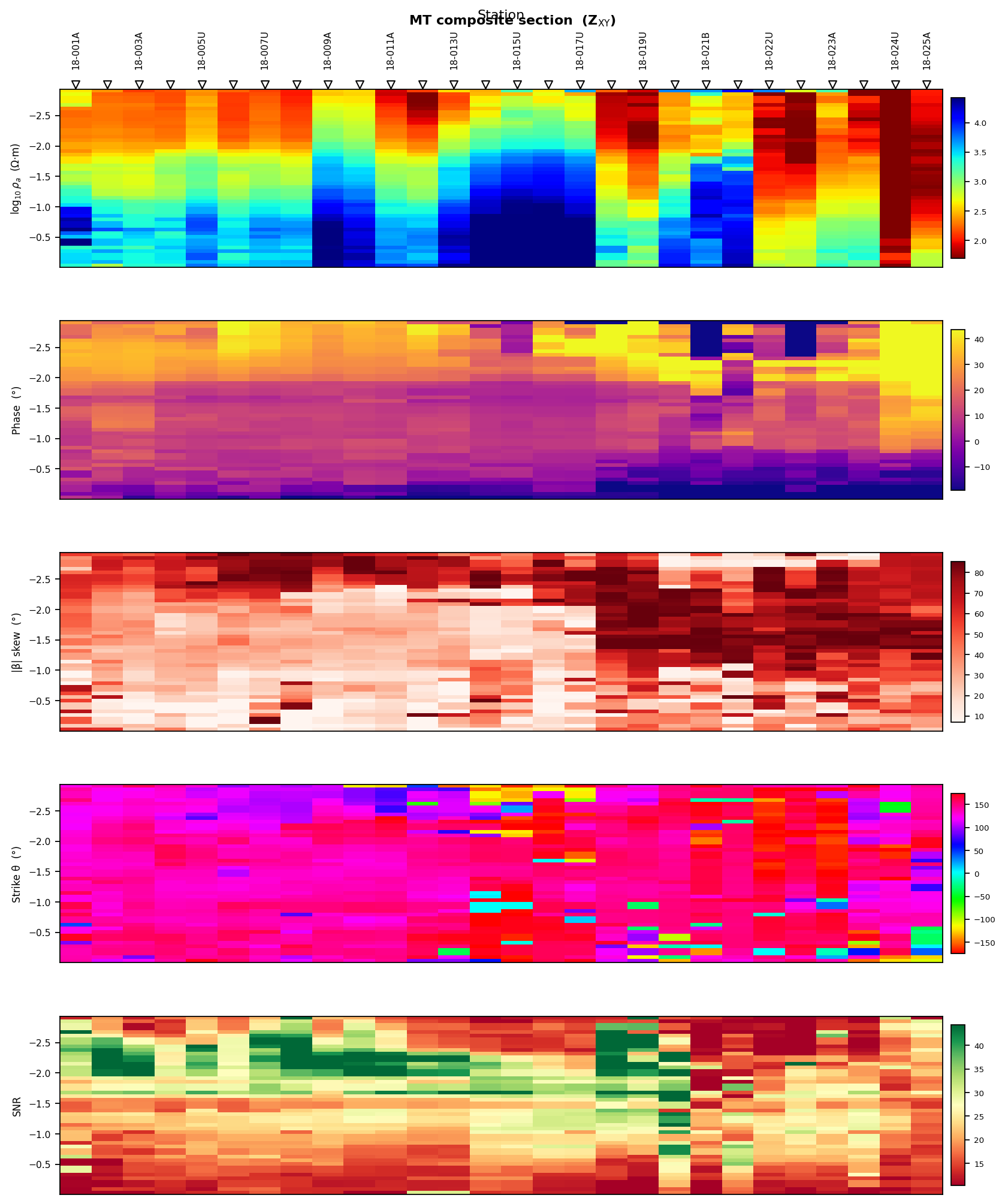
This is a compact report figure. It helps catch suspicious interpretations because rho, phase, skew, strike, and SNR are viewed on the same grid.

11.25.8.14. SNR Section

plot_snr_section() displays SNR by station, period, and component. It computes SNR as abs(Z) / abs(Z_err) when impedance errors are available, gives each selected component its own panel, and marks snr_thresh with a contour. For component \(Z_{ij}\), the plotted quantity is

\[\mathrm{SNR}_{ij} = {|Z_{ij}| \over |\sigma_{Z_{ij}}|+\varepsilon}.\]

When no impedance-error array is available, the function fills the corresponding cells with NaN rather than inventing a confidence estimate.

Key parameters

components usually includes ("xy", "yx"); snr_thresh sets the review threshold; vmax clips high-SNR cells so structure near the threshold remains visible.

>>> from pycsamt.emtools.advanced import plot_snr_section
>>> fig = plot_snr_section(
...     sites,
...     components=("xy", "yx"),
...     snr_thresh=3.0,
...     vmax=10.0,
...     recursive=False,
... )
>>> fig.savefig(out / "snr_section.png", dpi=200)

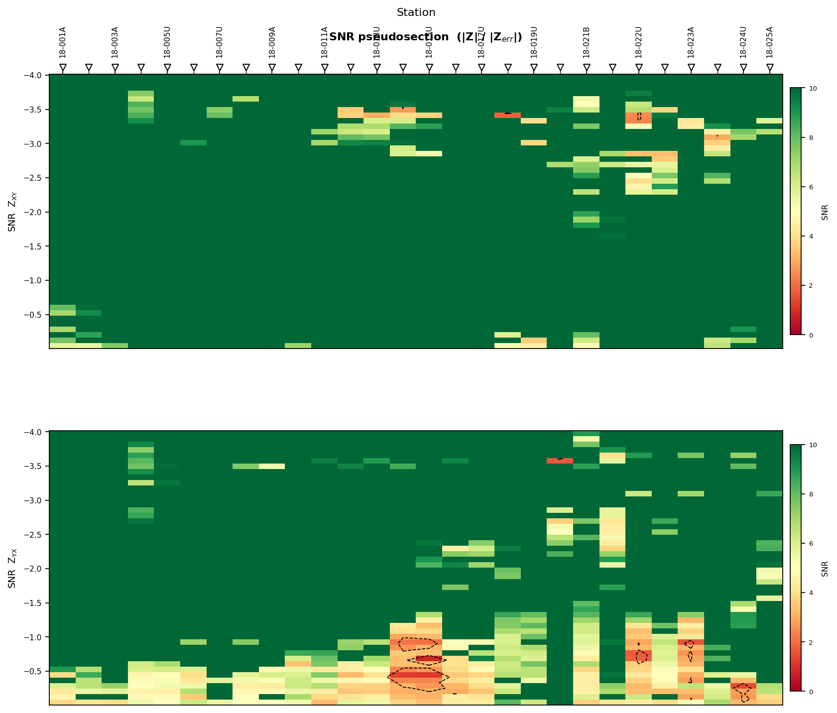
Cells below the threshold contour should be treated cautiously. If an entire frequency band has poor SNR, avoid over-interpreting that band.

11.25.8.15. Strike-Stability Bands

plot_strike_stability_bands() compares strike estimates across period and method. It computes or collects multiple strike indicators and plots period-dependent bands so method agreement and period stability are visible together. Because strike is axial, agreement is evaluated with wrapped angular differences,

\[\Delta\theta = ((\theta_1-\theta_2+90^\circ)\bmod 180^\circ)-90^\circ,\]

and the consensus band marks periods where methods fall within agreement_tol degrees on this axial scale.

Key parameters

methods chooses strike estimators; period_range isolates a band. Use this after basic phase-tensor and dimensionality checks.

>>> from pycsamt.emtools.advanced import plot_strike_stability_bands
>>> fig = plot_strike_stability_bands(
...     sites,
...     methods=("pt", "swift", "bahr"),
...     period_range=(1e-3, 10.0),
...     recursive=False,
... )
>>> fig.savefig(out / "strike_stability.png", dpi=200)

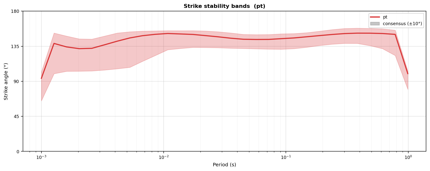
Stable overlapping bands support a consistent strike direction. Wide bands or disagreement between methods suggest 3-D structure, distortion, or an unsuitable period band.

11.25.8.16. Transfer-Function Coherence Network

plot_tf_coherence_network() visualizes station-to-station similarity using transfer-function curves. Stations are placed at their coordinates; the function interpolates log-apparent-resistivity curves onto a common period grid, computes Pearson correlation for station pairs, and draws edges for correlations above threshold. For station \(s\), let \(\mathbf{r}_s\) be the interpolated \(\log_{10}\rho_a(T)\) vector – an edge is then drawn when

\[\operatorname{corr}(\mathbf{r}_s,\mathbf{r}_t) \ge \tau,\]

where \(\tau\) is threshold. The network therefore compares curve shape over the selected band, not a single period sample.

Key parameters

component chooses the mode; threshold sets minimum correlation; max_edges prevents unreadable graphs; node_c_by colors nodes by a station summary metric such as skew, ellipticity, or resistivity; figsize overrides the automatic geographic aspect ratio, which is worth doing for a near-linear survey like L18PLT.

>>> from pycsamt.emtools.advanced import plot_tf_coherence_network
>>> fig = plot_tf_coherence_network(
...     sites,
...     component="xy",
...     period_range=(1e-3, 10.0),
...     threshold=0.90,
...     max_edges=120,
...     node_c_by="skew",
...     figsize=(7.5, 9.5),
...     recursive=False,
... )
>>> fig.savefig(out / "tf_coherence_network.png", dpi=200)

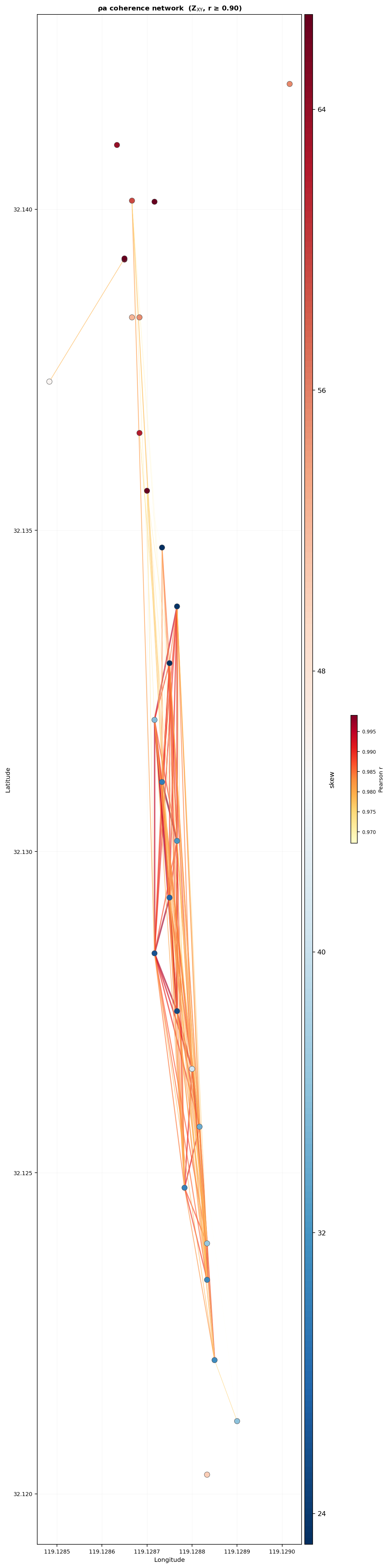
This function requires finite station coordinates. Isolated stations may be outliers, locally distorted, poorly located, or geologically distinct.

11.25.8.17. Embedding Advanced Plots

Most functions accept ax or axes so you can assemble multi-panel report figures.

>>> import matplotlib.pyplot as plt
>>> from pycsamt.emtools.advanced import plot_rho_phase_bode, plot_snr_section
>>> fig, axes = plt.subplots(3, 1, figsize=(9, 10))
>>> _ = plot_rho_phase_bode(
...     sites,
...     station="18-001A",
...     component="xy",
...     axes=axes[:2],
...     recursive=False,
... )
>>> _ = plot_snr_section(
...     sites,
...     components=("xy",),
...     axes=[axes[2]],
...     recursive=False,
... )
>>> fig.savefig(out / "advanced_report_panel.png", dpi=200)

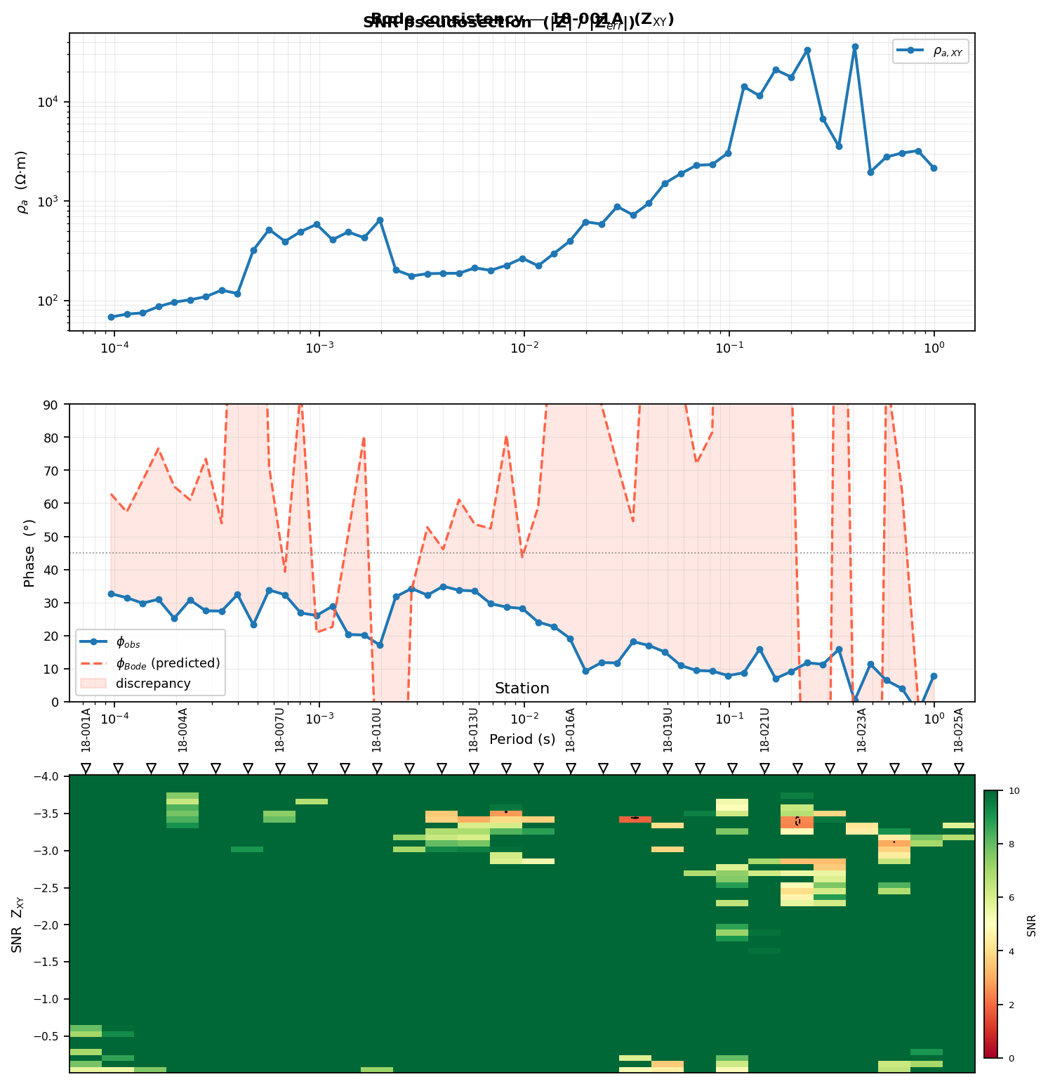
If you supply axes, the count must match the function. For example, plot_rho_phase_bode needs two axes, and plot_z_invariants_section needs four, as confirmed above with len(fig.axes).

11.25.8.18. Failure Modes And Checks

No impedance data

Check that files contain valid Z blocks and that ensure_sites did not skip all stations.

No phase-tensor data

Phase-tensor diagnostics require finite impedance components.

No coordinates

plot_tf_coherence_network requires finite station coordinates.

Crowded labels

Increase figsize, pass a station subset, or save at higher DPI.

Weak period bands

Compare advanced plots with QC and SNR figures. A coherent-looking pattern in a low-SNR band is weak evidence.

11.25.9. Worked Example

The full Sphinx-gallery example runs the advanced functions on the repository’s L18PLT example survey (data/AMT/WILLY_DATA/L18PLT). It starts with single-station tensor diagnostics, then moves through dimensionality, distortion, pseudosections, survey fingerprints, SNR, strike stability, and the transfer-function coherence network.

Open the rendered gallery page here: Novel MT visualizations (pycsamt.emtools.advanced).