
11.1. First-Look Survey Inspection#
pycsamt.emtools.inspect is the first module to use after loading a
survey. It answers practical questions before you run deeper
diagnostics, static shift correction, dimensionality
analysis, or inversion:
which stations loaded correctly?
which stations have impedance and tipper data?
do all stations share the same frequency grid?
are the apparent resistivity and phase curves sensible?
where are the first obvious pseudo-section anomalies?
which single station deserves a full response plot?
Full callable signatures live in the API reference. This page explains the workflow and gives concrete code patterns.
11.1.1. Why Inspect First#
Inspection is not interpretation yet. It is the quality gate between “the files loaded” and “the data are ready for scientific decisions”. The inspection tools are intentionally plain: tables, coverage masks, simple curves, pseudo-sections, tipper components, and one complete station dashboard.
The guiding idea is to separate existence from trust. A frequency sample can be present, finite, and plottable, while still being noisy, distorted, or inconsistent with neighboring stations. Inspection therefore answers the first question, “what do we actually have?”, and leaves stronger claims to the QC, tensor, skew, strike, and correction tools.
Run this stage before:
deciding which frequency band to keep;
comparing survey lines;
trusting tipper-based induction arrows;
building phase tensor or dimensionality products;
fitting a model response to observed data.
11.1.2. Load The Survey#
The inspection functions all call ensure_sites internally, but it is
still useful to normalize once at the top of a script.
>>> from pathlib import Path
>>> from pycsamt.emtools import ensure_sites
>>> edi_dir = Path("data/AMT/WILLY_DATA/L18PLT")
>>> survey = ensure_sites(
...     edi_dir,
...     recursive=True,
...     on_dup="replace",
...     strict=True,
...     verbose=1,
... )
Use strict=True when a missing or empty dataset should stop the
workflow. For exploratory notebooks, strict=False can be more
convenient because the plotting functions will draw “no data” messages
instead of failing immediately.
11.1.3. The Inspection Workflow#
The module is easiest to use as a sequence.
Step |
Question |
Tool |
|---|---|---|
inventory |
What stations, period ranges, coordinates, and tippers exist? |
|
required sections |
Which stations are missing |
|
frequency grid |
Do stations share the same frequency samples? |
|
quick curves |
Are rho/phase curves plausible? |
|
survey image |
Where are station-period anomalies? |
|
tipper check |
Is real tipper present and stable? |
|
station dashboard |
What does one station look like in full? |
|
11.1.4. Per-Site Summary#
sites_summary returns one row per station. By default it reports
station name, number of frequency samples, whether tipper data are
present, period range, and coordinates.
For station \(s\), the summary period limits are computed from its frequency vector \(\{f_{s,j}\}\):
The has_tipper flag is not a plain attribute check. It uses the
same transfer-function extraction path used by the plotting tools, so a
placeholder tipper object is not counted unless usable tipper samples
are present.
>>> import pandas as pd
>>> from pycsamt.emtools import ensure_sites, sites_summary
>>> survey = ensure_sites("data/AMT/WILLY_DATA/L18PLT", strict=True)
>>> summary = sites_summary(survey, api=False)
>>> summary.head()
   station  n_freq  has_tipper  period_min  period_max        lat         lon
0  18-001A      53       False    0.000096    0.992063  32.120300  119.128833
1  18-002U      53       False    0.000096    0.992063  32.121133  119.128900
2  18-003A      53       False    0.000096    0.992063  32.122083  119.128850
3  18-004A      53       False    0.000096    0.992063  32.123333  119.128833
4  18-005U      53       False    0.000096    0.992063  32.123900  119.128833
>>> overview = {
...     "n_sites": len(summary),
...     "has_any_tipper": bool(summary["has_tipper"].any()),
...     "n_freq_values": sorted(summary["n_freq"].unique()),
...     "period_min": float(summary["period_min"].min()),
...     "period_max": float(summary["period_max"].max()),
... }
>>> pd.Series(overview)
n_sites                 28
has_any_tipper       False
n_freq_values         [53]
period_min        0.000096
period_max        0.992063
dtype: object
Read this table before plotting anything. A survey with mixed
n_freq values needs frequency-grid attention. A survey with
has_tipper=False everywhere should not be sent into tipper or
induction-arrow interpretation.
11.1.5. Choose Summary Columns#
The fields argument lets you keep the inventory narrow when you are
printing reports or comparing several lines.
>>> from pycsamt.emtools import sites_summary
>>> compact = sites_summary(
...     "data/AMT/WILLY_DATA/L18PLT",
...     fields=(
...         "station",
...         "n_freq",
...         "period_min",
...         "period_max",
...         "has_tipper",
...     ),
...     api=False,
... )
>>> print(compact.to_string(index=False))
station  n_freq  period_min  period_max  has_tipper
18-001A      53    0.000096    0.992063       False
18-002U      53    0.000096    0.992063       False
18-003A      53    0.000096    0.992063       False
18-004A      53    0.000096    0.992063       False
18-005U      53    0.000096    0.992063       False
18-006A      53    0.000096    0.992063       False
18-007U      53    0.000096    0.992063       False
18-008U      53    0.000096    0.992063       False
18-009A      53    0.000096    0.992063       False
18-010U      53    0.000096    0.992063       False
18-011A      53    0.000096    0.992063       False
18-012A      53    0.000096    0.992063       False
18-013U      53    0.000096    0.992063       False
18-014A      53    0.000096    0.992063       False
18-015U      53    0.000096    0.992063       False
18-016A      53    0.000096    0.992063       False
18-017U      53    0.000096    0.992063       False
18-018A      53    0.000096    0.992063       False
18-019U      53    0.000096    0.992063       False
18-020A      53    0.000096    0.992063       False
18-021U      53    0.000096    0.992063       False
18-021B      53    0.000096    0.992063       False
18-022U      53    0.000096    0.992063       False
18-022V      53    0.000096    0.992063       False
18-023A      53    0.000096    0.992063       False
18-023V      53    0.000096    0.992063       False
18-024U      53    0.000096    0.992063       False
18-025A      53    0.000096    0.992063       False
The returned object may be an API-aware frame when the package API-view
mode is enabled. Passing api=False gives a plain pandas
DataFrame for ordinary scripts.
11.1.6. Missing Sections#
list_missing_sections checks whether each station has required data
sections. The most common checks are "mt" for impedance and
"tipper" for transfer-function data.
>>> from pycsamt.emtools import ensure_sites, list_missing_sections
>>> survey = ensure_sites("data/AMT/WILLY_DATA/L18PLT", strict=True)
>>> missing = list_missing_sections(
...     survey,
...     require=("mt", "tipper"),
... )
>>> for station, sections in missing.items():
...     print(f"{station}: missing {', '.join(sections)}")
...
18-001A: missing tipper
18-002U: missing tipper
18-003A: missing tipper
18-004A: missing tipper
18-005U: missing tipper
18-006A: missing tipper
18-007U: missing tipper
18-008U: missing tipper
18-009A: missing tipper
18-010U: missing tipper
18-011A: missing tipper
18-012A: missing tipper
18-013U: missing tipper
18-014A: missing tipper
18-015U: missing tipper
18-016A: missing tipper
18-017U: missing tipper
18-018A: missing tipper
18-019U: missing tipper
18-020A: missing tipper
18-021U: missing tipper
18-021B: missing tipper
18-022U: missing tipper
18-022V: missing tipper
18-023A: missing tipper
18-023V: missing tipper
18-024U: missing tipper
18-025A: missing tipper
This function uses the same internal extraction helpers as the plotting tools. That matters because real EDI/Site objects can expose placeholder attributes even when a section was not actually parsed.
11.1.7. Check Tipper Availability Explicitly#
AMT/CSAMT lines often have no tipper. MT surveys often do. Make that difference explicit before writing code that assumes tipper exists.
>>> amt_missing = list_missing_sections(
...     "data/AMT/WILLY_DATA/L18PLT",
...     require=("tipper",),
... )
>>> mt_missing = list_missing_sections(
...     "data/MT/kap03lmt_edis",
...     require=("tipper",),
... )
>>> print(f"L18PLT stations missing tipper: {len(amt_missing)}")
L18PLT stations missing tipper: 28
>>> print(f"KAP03 stations missing tipper: {len(mt_missing)}")
KAP03 stations missing tipper: 0
If every station is missing tipper, that is not necessarily a failure. It simply means you should stay with impedance-based inspection and use the transfer-function tools only on surveys that contain vertical-field data.
11.1.8. Frequency Coverage Tables#
frequency_coverage has three modes.
For station \(s\), let \(F_s\) be its set of valid positive frequencies. The survey union and intersection are
mode="per-site" returns the individual \(F_s\) arrays,
mode="union" returns \(F_\cup\), and mode="intersection"
returns \(F_\cap\). A large union with an empty or tiny
intersection means the survey needs frequency-grid alignment before
station-by-station comparisons are treated as common-period statistics.
>>> import numpy as np
>>> from pycsamt.emtools import ensure_sites, frequency_coverage
>>> survey = ensure_sites("data/MT/kap03lmt_edis", strict=True)
>>> per_site = frequency_coverage(survey, mode="per-site")
>>> union = frequency_coverage(survey, mode="union")
>>> intersection = frequency_coverage(survey, mode="intersection")
>>> print(f"stations: {len(per_site)}")
stations: 26
>>> print(f"union frequency count: {union.size}")
union frequency count: 37
>>> print(f"common frequency count: {intersection.size}")
common frequency count: 0
>>> for station, freq in per_site.items():
...     missing_from_union = np.setdiff1d(union, freq)
...     if missing_from_union.size:
...         print(station, "missing", missing_from_union.size, "samples")
...
kap103 missing 17 samples
kap106 missing 17 samples
kap109 missing 20 samples
kap112 missing 17 samples
kap115 missing 17 samples
kap118 missing 17 samples
kap121 missing 17 samples
kap123 missing 17 samples
kap125 missing 17 samples
kap127 missing 17 samples
kap130 missing 17 samples
kap133 missing 17 samples
kap136 missing 17 samples
kap139 missing 17 samples
kap142 missing 17 samples
kap145 missing 19 samples
kap148 missing 17 samples
kap151 missing 17 samples
kap152 missing 17 samples
kap155 missing 17 samples
kap157 missing 17 samples
kap160 missing 17 samples
kap163 missing 17 samples
kap169 missing 17 samples
kap172 missing 17 samples
kap175 missing 17 samples
Use mode="per-site" when you need station names. Use "union"
to know the full survey frequency grid. Use "intersection" to know
which frequencies are shared by every station.
11.1.9. Plot Frequency Coverage#
For a first-pass acquisition dashboard, combine row counts and frequency
placement with plot_survey_inventory_overview(). Its
station markers and labels sit above the count profile, while the lower map
uses the same station centres to expose missing bands that equal row counts
could conceal:
>>> from pycsamt.emtools import plot_survey_inventory_overview
>>> fig = plot_survey_inventory_overview(
...     survey,
...     station_grid=True,
...     station_grid_kws={"color": "white", "linestyle": ":"},
... )
Use count_kws to control the upper line and markers, coverage_cmap for
the lower map, and station_labels when display names should be shorter
than the identifiers retained in the data.
plot_coverage converts the frequency dictionary into a station by
frequency presence mask.
On the union grid \(F_\cup=\{g_i\}\), the plotted mask is
The image therefore shows data availability only. It does not know whether the impedance estimate at that frequency is stable, low-noise, or geologically reasonable.
>>> import matplotlib.pyplot as plt
>>> from pycsamt.emtools import plot_coverage
>>> fig, ax = plt.subplots(figsize=(8.0, 4.5))
>>> _ = plot_coverage(
...     survey,
...     axis="period",
...     ax=ax,
... )
>>> _ = ax.set_title("KAP03 frequency coverage")
>>> fig.tight_layout()
>>> fig.savefig("kap03_frequency_coverage.png", dpi=200)
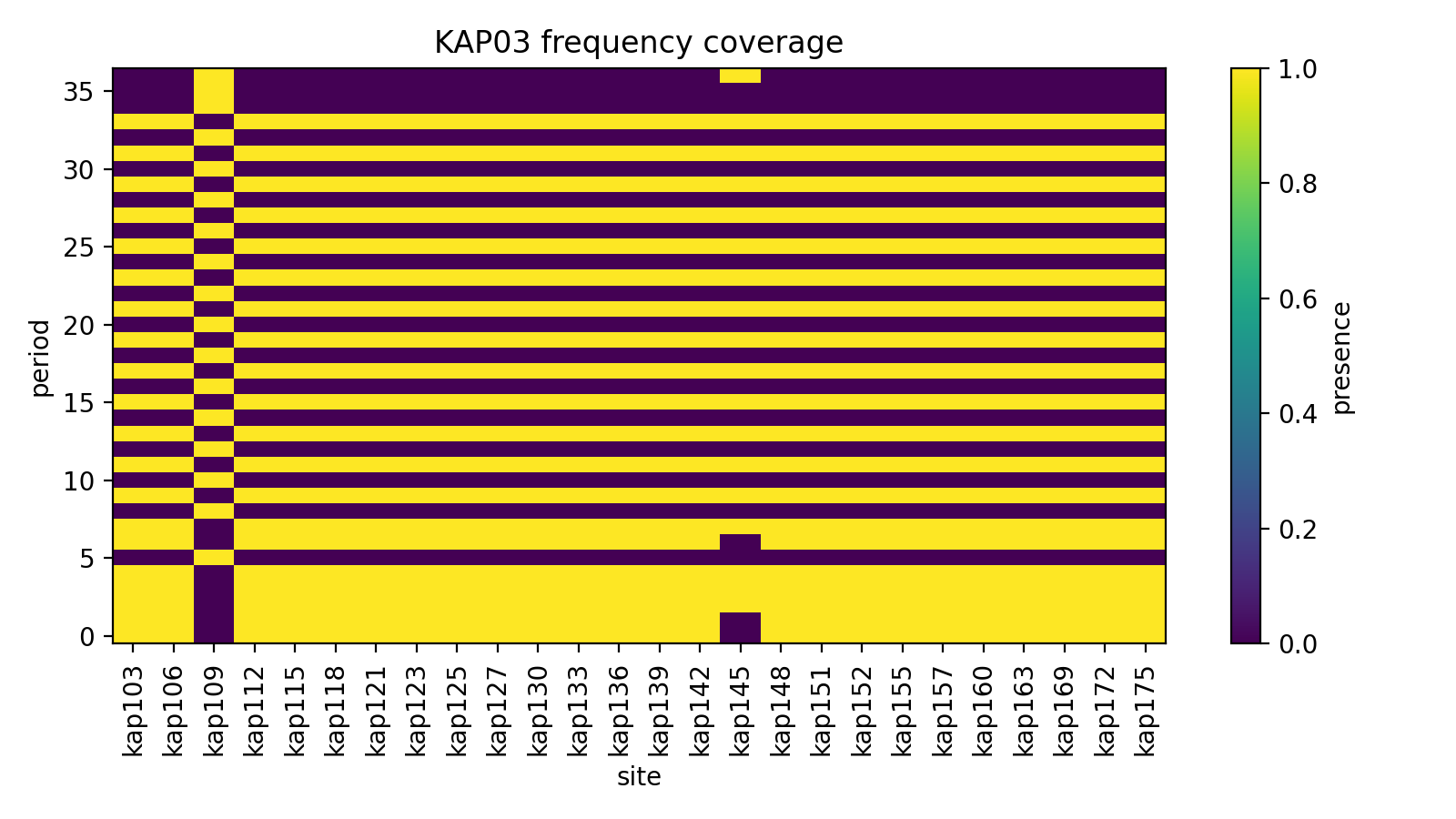
The colour value is presence, not data quality. A fully covered cell only means the sample exists. Use QC, error, confidence, and frequency editing tools to decide whether the sample is reliable.
11.1.10. Quick Rho And Phase Curves#
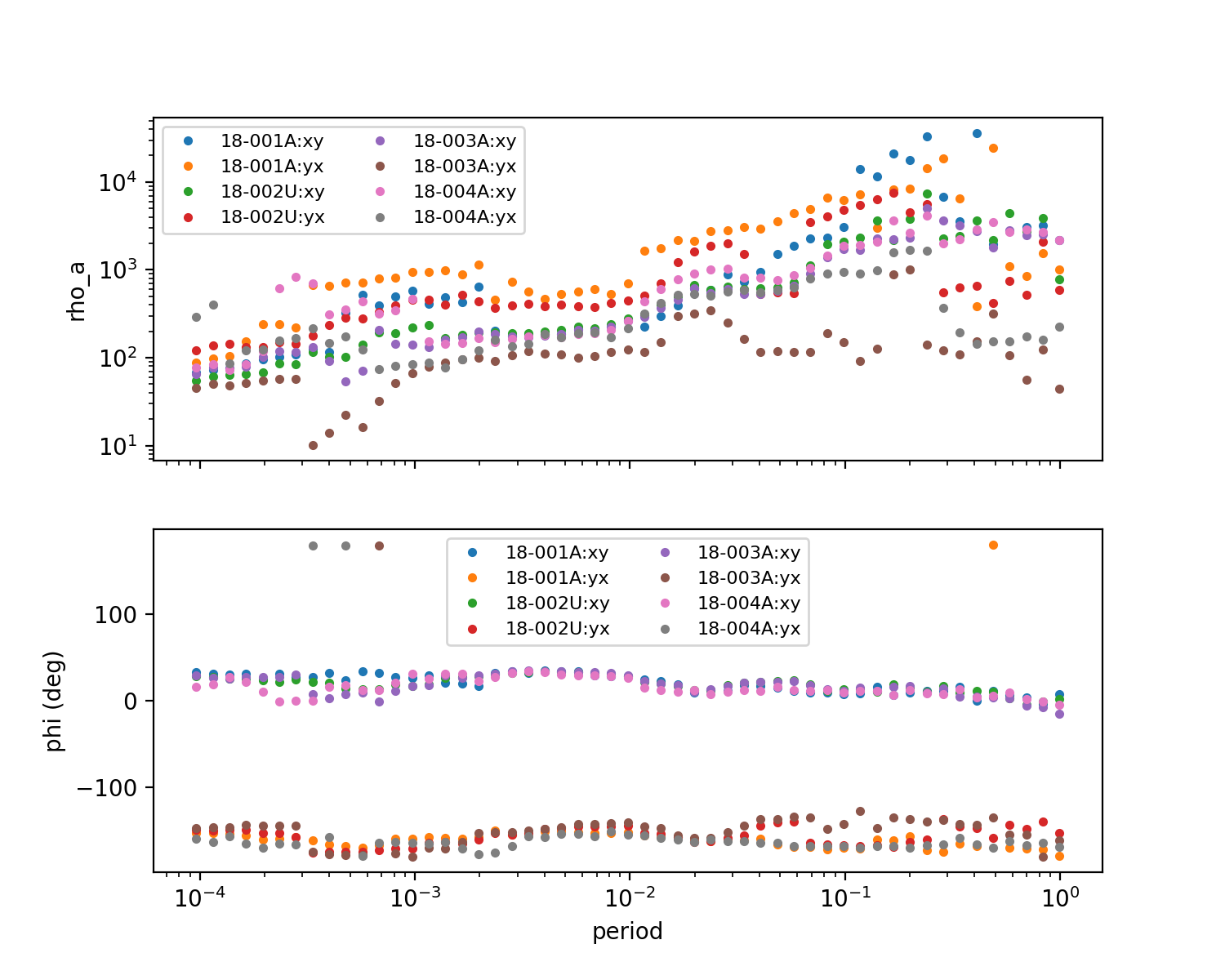
plot_rhoa_phi plots apparent resistivity and phase for one or more
stations. It accepts components such as "xy", "yx", "xx",
and "yy" when those columns exist in the station dataframe.
For an impedance component \(Z_{ij}(f)\), the displayed quantities are
Resistivity is drawn on logarithmic axes because multiplicative shifts and band-limited anomalies are easier to compare by ratio than by absolute difference. Phase stays in degrees, so jumps, wraps, or component sign conventions should be checked before reading them as smooth physical trends.
>>> from pycsamt.emtools import plot_rhoa_phi
>>> from pycsamt.emtools._core import _iter_items
>>> survey = ensure_sites("data/AMT/WILLY_DATA/L18PLT", strict=True)
>>> subset_paths = [site.edi.path for site in list(_iter_items(survey))[:4]]
>>> subset = ensure_sites(subset_paths, strict=True)
>>> ax_rho, ax_phase = plot_rhoa_phi(
...     subset,
...     components=("xy", "yx"),
...     axis="period",
...     errorbar=True,
...     figsize=(8.0, 6.0),
... )
>>> ax_rho.figure.savefig("l18plt_rho_phase_subset.png", dpi=200)
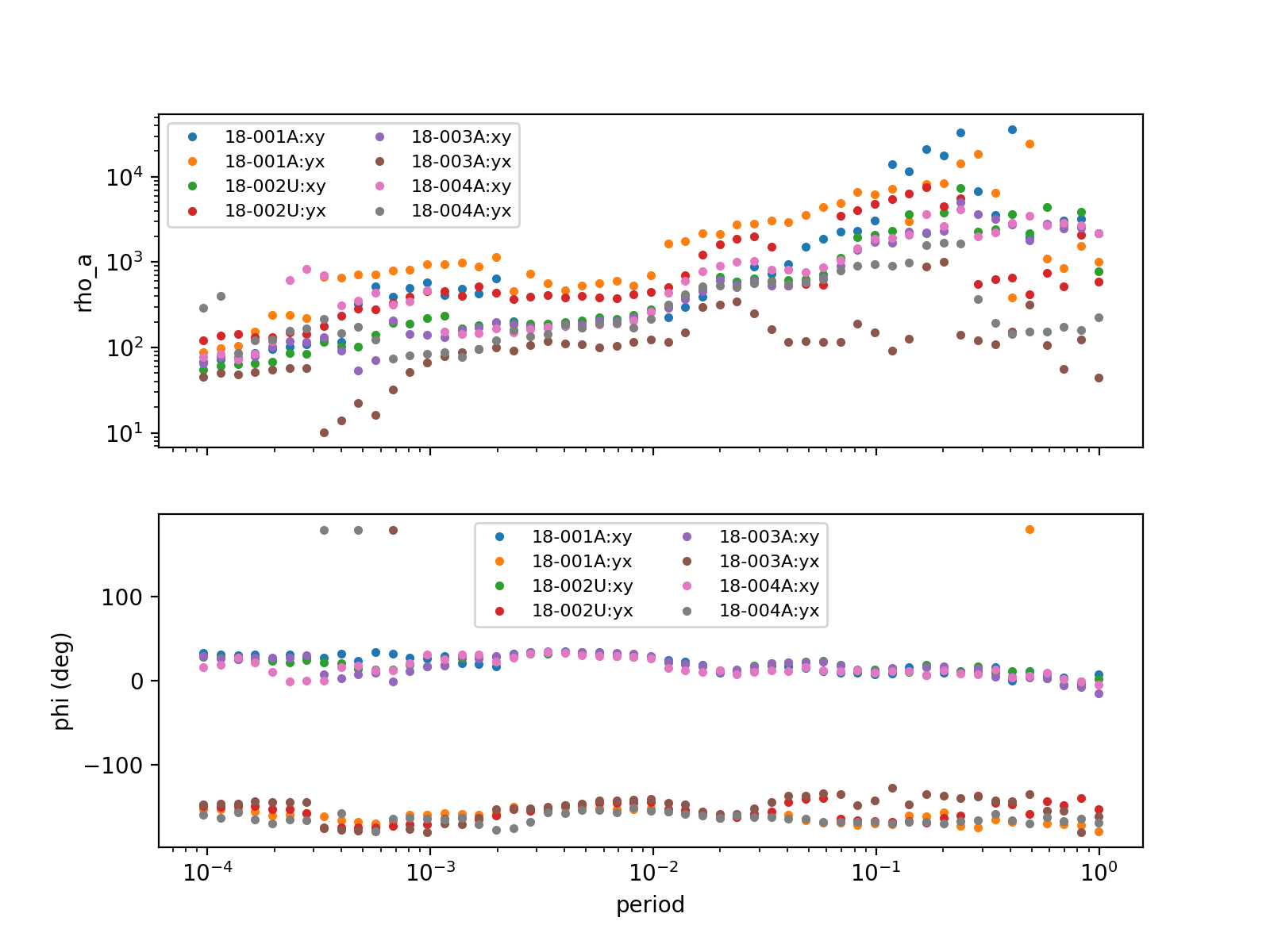
Do not plot every station at once unless the survey is tiny. The
function will draw the data, but the legend can become unreadable. Use
small station subsets for first inspection, then switch to
plot_station_response for a station-level deep view.
11.1.11. Pseudo-Sections#
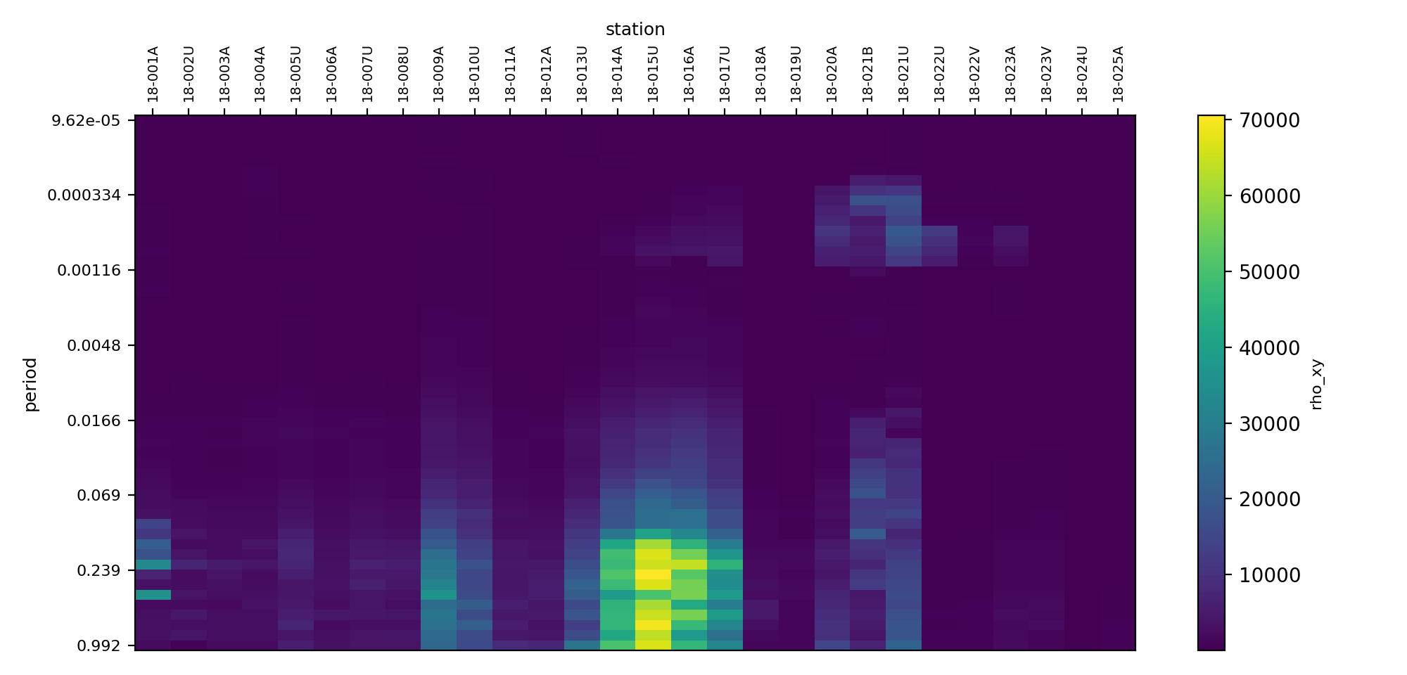
pseudosection creates a period by station image from a dataframe
quantity such as "rho_xy", "rho_yx", "phi_xy", or
"phi_yx". Values are pivoted by station and period, with median
aggregation for duplicate cells.
For quantity \(q\), station \(s\), and period \(T\), the cell value is
The median aggregation is defensive: if duplicate rows exist after loading or merging, one repeated value cannot dominate the cell by counting more than once in a mean.
>>> from pycsamt.emtools import pseudosection
>>> fig, ax = plt.subplots(figsize=(10.0, 4.8))
>>> _ = pseudosection(
...     survey,
...     quantity="rho_xy",
...     period_range=(1e-4, 1.0),
...     ax=ax,
...     topo=False,
... )
>>> _ = ax.set_title("L18PLT rho_xy pseudo-section")
>>> fig.tight_layout()
>>> fig.savefig("l18plt_rho_xy_pseudosection.png", dpi=200)
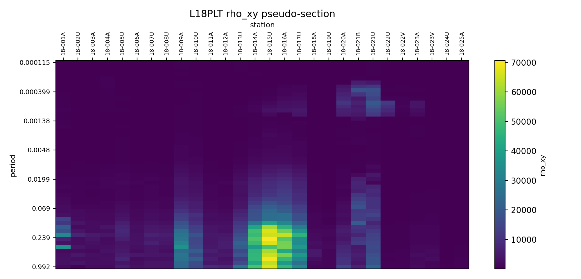
The x-axis is station order. The y-axis is period. Short periods are drawn at the top because the image uses the common MT pseudo-section convention: shallow-sensitive samples above deeper-sensitive samples.
11.1.12. Control The Pseudo-Section Scale#
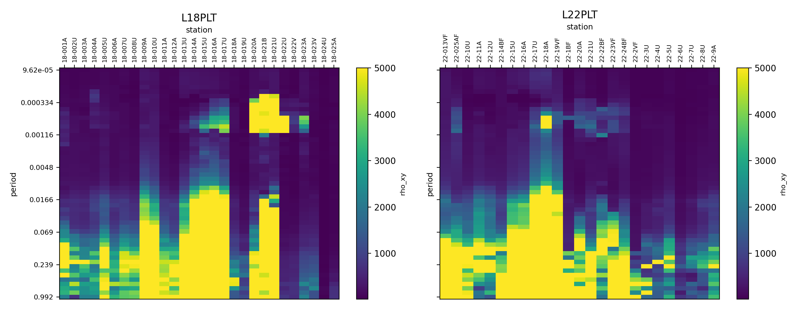
Use fixed vmin and vmax when comparing two lines. Otherwise a
line with a narrow value range can look as dramatic as a line with a
much stronger anomaly.
For two lines \(A\) and \(B\), use one shared color transform \(C(q; v_\min, v_\max)\). Otherwise each panel silently rescales its own values and a weak anomaly on one line can appear visually equal to a much stronger anomaly on another.
>>> line18 = ensure_sites("data/AMT/WILLY_DATA/L18PLT", strict=True)
>>> line22 = ensure_sites("data/AMT/WILLY_DATA/L22PLT", strict=True)
>>> fig, axes = plt.subplots(1, 2, figsize=(13.0, 5.0), sharey=True)
>>> _ = pseudosection(line18, quantity="rho_xy", vmin=10.0, vmax=5000.0, ax=axes[0])
>>> _ = axes[0].set_title("L18PLT")
>>> _ = pseudosection(line22, quantity="rho_xy", vmin=10.0, vmax=5000.0, ax=axes[1])
>>> _ = axes[1].set_title("L22PLT")
>>> fig.tight_layout()
>>> fig.savefig("rho_xy_line_comparison.png", dpi=200)
If topography is configured globally, pseudosection can draw an
optional topography strip. Pass topo=False when you want a compact
data-only panel.
11.1.13. Resistivity and Phase Pseudo-Sections#
pseudosection draws one quantity at a time. When you want the
familiar MT layout – apparent resistivity stacked above phase, one
column per impedance tensor component, every panel sharing the
period axis and one colour scale –
PlotResPhasePseudoSection assembles the whole
figure in a single call.
Each station’s samples are snapped onto a log-spaced period grid of
\(N\) rows (n_grid, default 60). For grid row \(T_k\) and
station \(s\) the cell takes the nearest observed period within
0.3 decades,
and is left blank when no sample falls inside the window, so gapped or
decimated stations stay visibly empty rather than being interpolated
across. The grid ends are set from the half-decade period bins in which
at least a fraction of the line’s stations carry data, so one file’s
stray high-frequency segment cannot stretch the axis across empty
decades. Resistivity is mapped as \(\log_{10}\rho_a\) by default;
the yx and yy phases are rotated by \(180^\circ\) so a 1-D
response plots near \(45^\circ\) in every column.
>>> from pycsamt.emtools import PlotResPhasePseudoSection
>>> survey = ensure_sites("data/AMT/WILLY_DATA/L18PLT", strict=True)
>>> len(survey)
28
>>> fig = PlotResPhasePseudoSection(
...     survey,
...     title="L18PLT -- apparent resistivity and phase",
... ).plot()
>>> fig.savefig("l18plt_res_phase_pseudosection.png", dpi=160)
With components=None every component that carries finite data is
detected and drawn in canonical xy, yx, xx, yy order; L18PLT is a
full-tensor line, so all four columns appear. The station names and the
inverted-triangle markers come from
PYCSAMT_STATION_RENDERING, so they match every
other pyCSAMT section view.
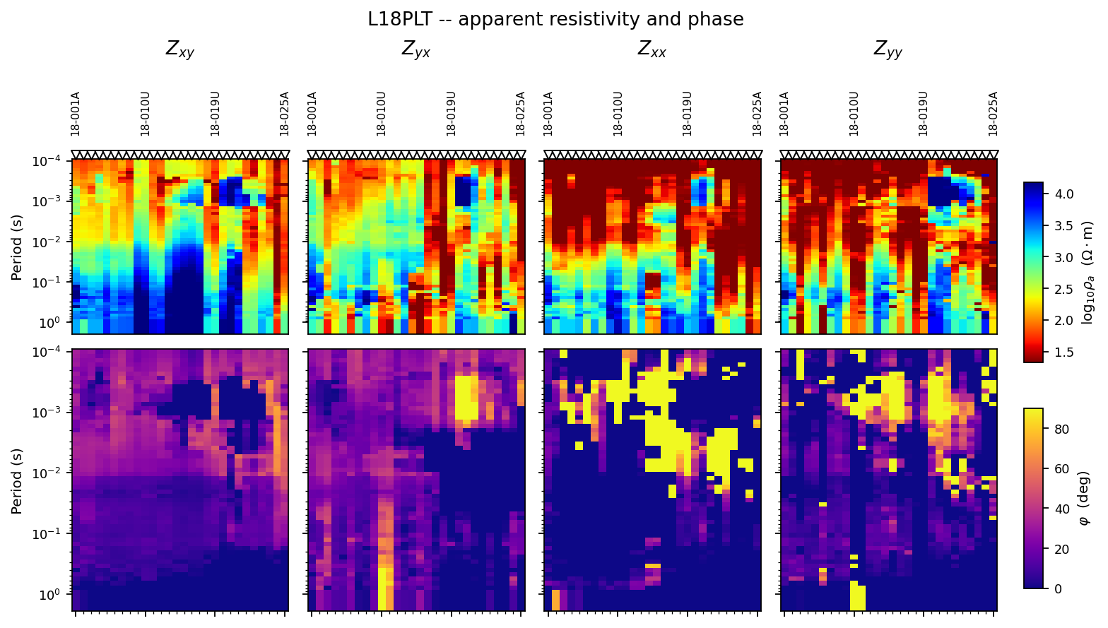
The off-diagonal columns (\(Z_{xy}\), \(Z_{yx}\)) carry the interpretable signal: a broad low-resistivity band that deepens toward one end of the line, with phase above \(45^\circ\) over the conductor and below it over resistive blocks. The diagonal columns (\(Z_{xx}\), \(Z_{yy}\)) are an order of magnitude weaker and mostly noise here – their phase saturates against the colour limits – which is itself the diagnostic: a quasi-1-D or 2-D site has small diagonal terms, and columns that light up coherently instead point to 3-D structure or a strike misalignment worth following up with the dimensionality and strike tools.
11.1.13.1. Panel Layout And The Station Axis#
res_phase_ratio sets the height of a resistivity panel relative to
its phase panel. The default \(2/3\) gives phase more room because
phase resolves lateral contacts sharply; pass 2.0 for the opposite
emphasis – resistivity fills two-thirds of the row-pair and phase the
remaining third – or 1.0 for equal panels. components also
fixes the column order: pass ["yx", "xy"] to lead with the TM-like
mode.
station_side controls where the station axis is drawn: "top"
(the default, matching the pyCSAMT section convention), "bottom",
or "none". station_markers=False keeps only the names.
panel_labels=True tags each row-pair (a), (b), …, and
grid=True adds faint period grid lines.
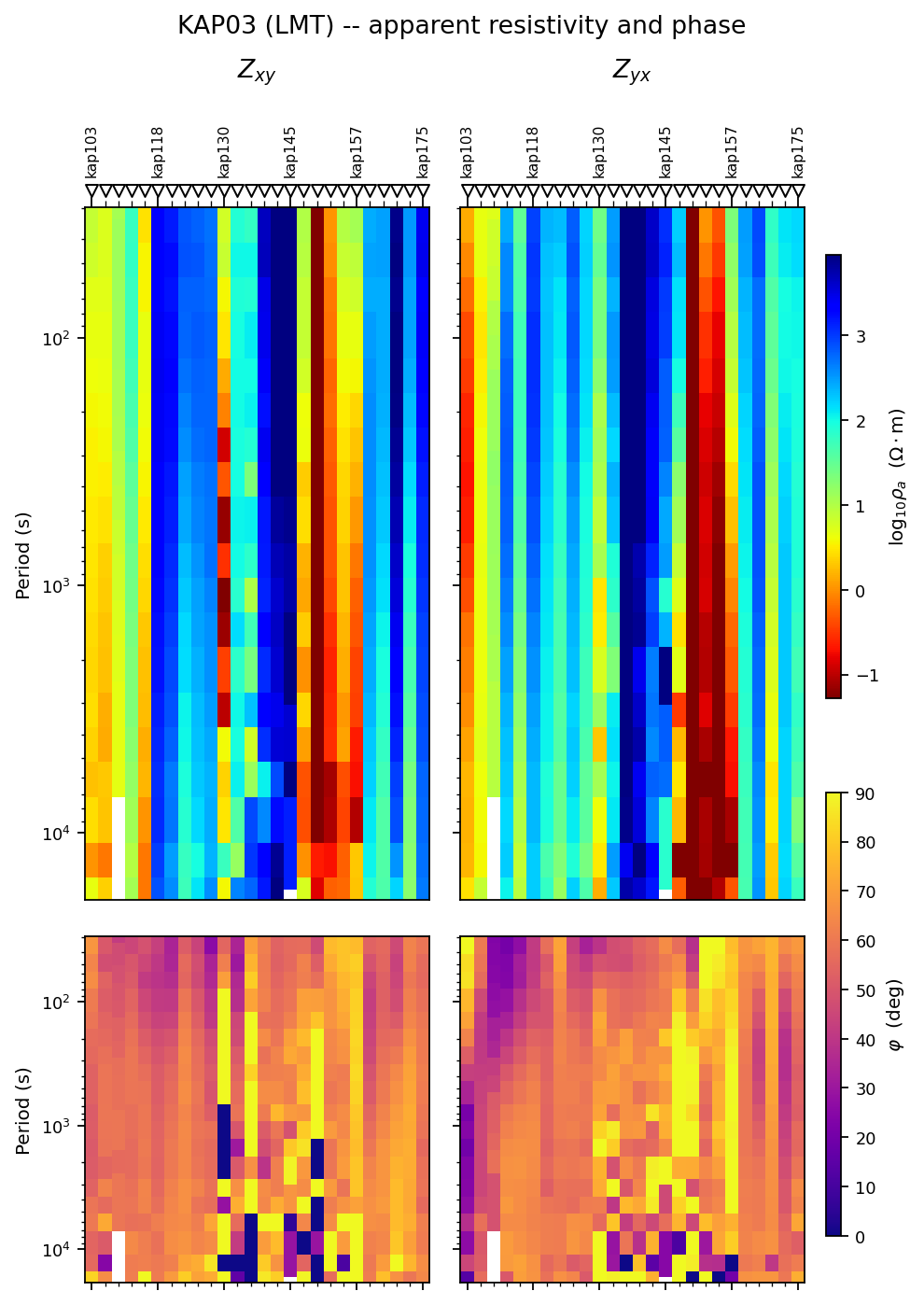
>>> kap03 = ensure_sites("data/MT/kap03lmt_edis", strict=True)
>>> len(kap03)
26
>>> fig = PlotResPhasePseudoSection(
...     kap03,
...     components=["xy", "yx"],
...     res_phase_ratio=2.0,
...     station_side="top",
...     title="KAP03 (LMT) -- apparent resistivity and phase",
... ).plot()
>>> fig.savefig("kap03_res_phase_pseudosection.png", dpi=160)
KAP03 is the bundled long-period (LMT) line from the MTPy sample data,
recorded between roughly 30 and 20 000 s. With resistivity given twice
the height of phase the deep structure dominates the figure: a
persistent low-resistivity zone under the central stations (kap145
to kap157) with phase pinned near \(90^\circ\), flanked by
resistive blocks where the phase drops below \(45^\circ\).
11.1.13.2. Stacking Several Lines#
Pass a mapping to stack lines as extra [resistivity, phase]
row-pairs, each with its own station axis. By default every pair is
resampled onto one shared period grid and shares one resistivity colour
scale (from the off-diagonal components) and one phase colour scale, so
the lines are directly comparable.
>>> line18 = ensure_sites("data/AMT/WILLY_DATA/L18PLT", strict=True)
>>> line22 = ensure_sites("data/AMT/WILLY_DATA/L22PLT", strict=True)
>>> fig = PlotResPhasePseudoSection(
...     {"L18PLT": line18, "L22PLT": line22},
...     components=["xy", "yx"],
...     panel_labels=True,
... ).plot()
>>> fig.savefig("willy_two_line_res_phase.png", dpi=160)
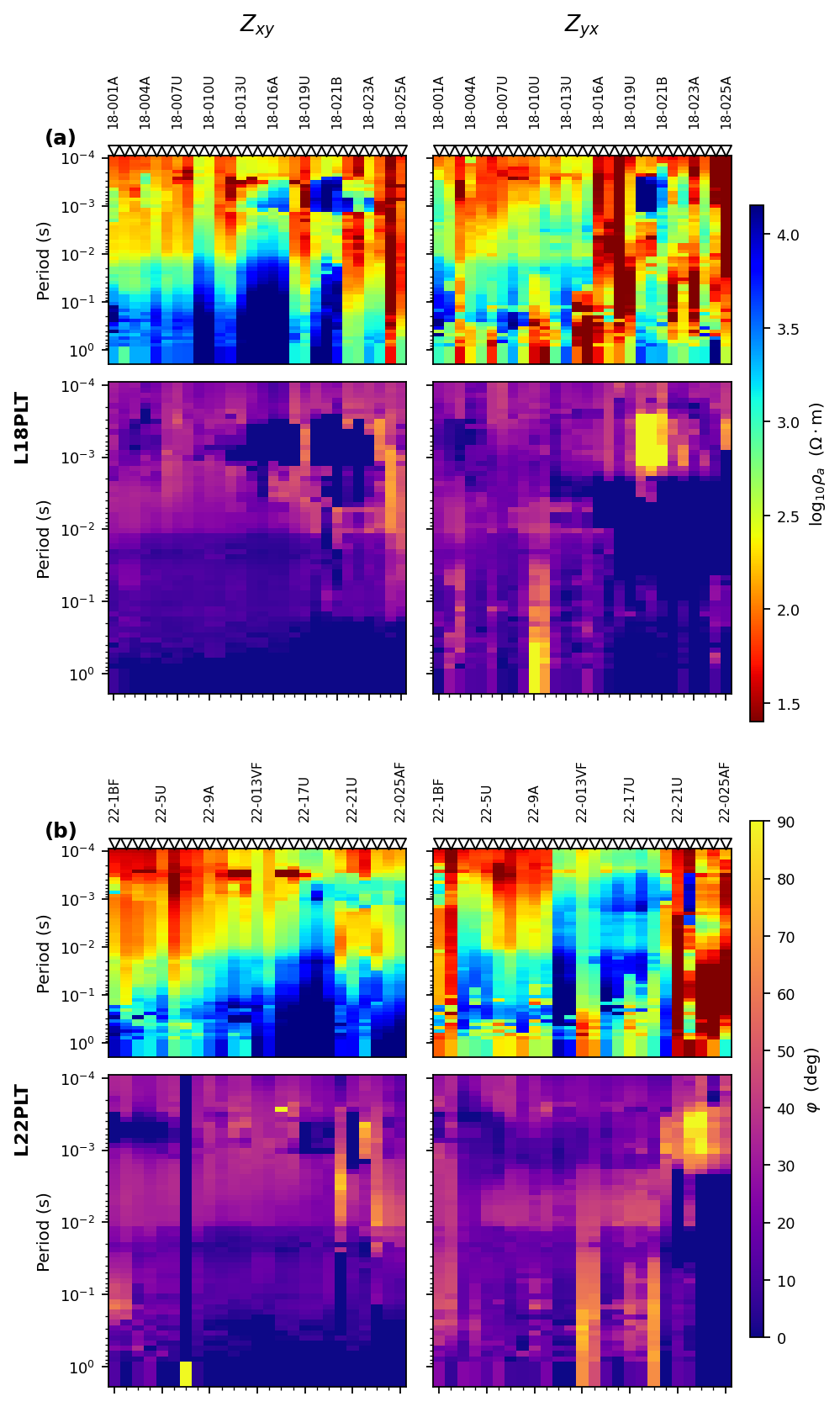
L18PLT and L22PLT are adjacent AMT lines over the same period band, so the shared axis and colour scale make the comparison immediate: both show a shallow resistive cap breaking down into a mid-period conductor, stronger and shallower under the northern half of L22PLT.
When the lines come from different instruments their period bands
barely overlap, and one shared axis wastes most of the figure. Set
share_period=False to give each group its own period window.
>>> fig = PlotResPhasePseudoSection(
...     {"KAP03 (LMT)": kap03, "L18PLT (AMT)": line18},
...     components=["xy", "yx"],
...     res_phase_ratio=2.0,
...     share_period=False,
...     panel_labels=True,
... ).plot()
>>> fig.savefig("kap03_l18_stacked.png", dpi=160)
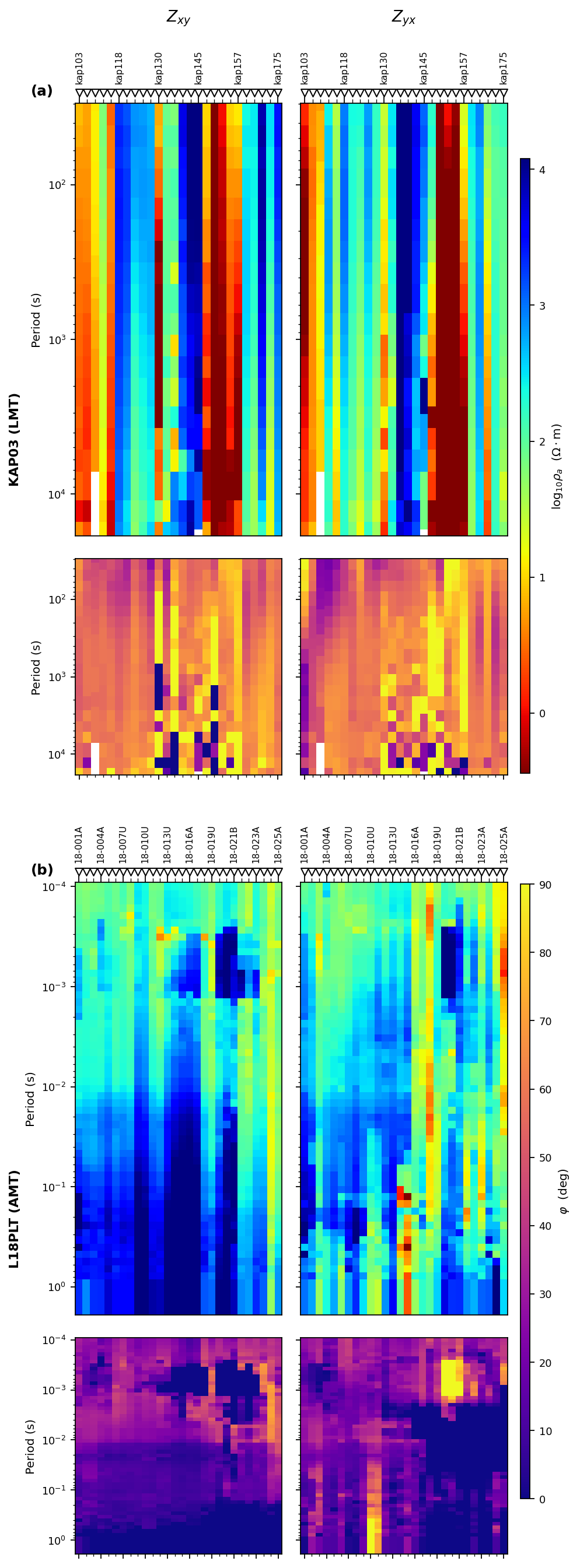
The long-period KAP03 conductor and the shallow, higher-frequency structure under L18PLT now each fill their own panel while still sharing one colour key.
phase_range accepts the presets "0-90" (default),
"-45-45", "-90-90", "-180-180", the string "auto"
(2nd/98th percentiles), or an explicit (vmin, vmax) tuple. A signed
window makes out-of-quadrant phases – 3-D effects, polarisation
overprint, or a bad station – stand out instead of being clipped to
the edge of a \(0\)–\(90^\circ\) scale.
11.1.14. Tipper Components#
plot_tipper_components draws real and imaginary parts of Tx and
Ty versus period or frequency. Use it only after confirming that
the survey actually contains tipper data.
The plotted curves are the four scalar tracks
The vector magnitude used later by transfer-function maps is \(|\mathbf{T}|=\sqrt{|T_x|^2+|T_y|^2}\), but this component view is often better for finding sign flips, isolated spikes, or a single component that is driving the whole anomaly.
>>> from pycsamt.emtools import plot_tipper_components
>>> from pycsamt.emtools._core import _name
>>> survey = ensure_sites("data/MT/kap03lmt_edis", strict=True)
>>> station_names = ["kap103", "kap121", "kap142", "kap151"]
>>> subset_paths = [
...     site.edi.path
...     for index, site in enumerate(_iter_items(survey))
...     if _name(site, index) in station_names
... ]
>>> subset = ensure_sites(subset_paths, strict=True)
>>> fig, ax = plt.subplots(figsize=(8.5, 4.8))
>>> _ = plot_tipper_components(
...     subset,
...     kind=("real", "imag"),
...     axis="period",
...     ax=ax,
... )
>>> _ = ax.set_title("KAP03 selected tipper components")
>>> fig.tight_layout()
>>> fig.savefig("kap03_tipper_components.png", dpi=200)
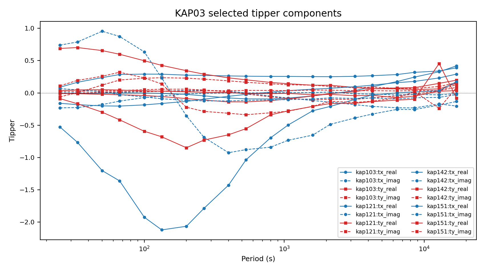
The horizontal zero line is important. Sign changes, isolated spikes, or one station separating strongly from the others are good reasons to inspect induction arrows, tipper hodograms, and station metadata.
11.1.15. Full Station Response#
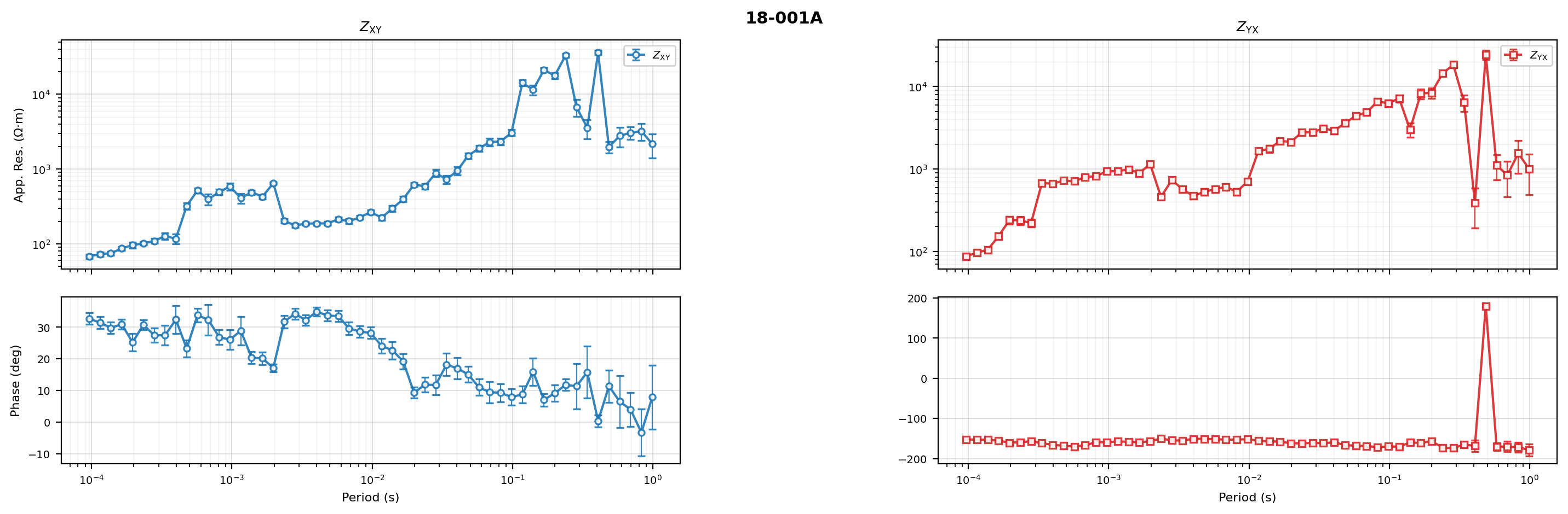
plot_station_response is the richest first-look figure. It shows
apparent resistivity, phase, and, when available, the four tipper
sub-panels for one station.
For each selected impedance component, the station response keeps the period mask explicit:
This matters because a station can look clean over one band and unstable
over another. Keep the plotted period_range close to the band you
will later use for inversion, strike, or dimensionality decisions.
>>> from pycsamt.emtools import plot_station_response
>>> survey = ensure_sites("data/MT/kap03lmt_edis", strict=True)
>>> fig = plot_station_response(
...     survey,
...     station="kap151",
...     components=("xx", "xy", "yx", "yy"),
...     period_range=(1e-2, 2e4),
...     show_tipper=True,
...     show_error_bars=True,
...     rho_lim=None,
...     phase_lim=None,
...     tipper_lim=(-2.5, 2.5),
...     title="kap151 first-look response",
... )
>>> fig.savefig("kap151_station_response.png", dpi=200)
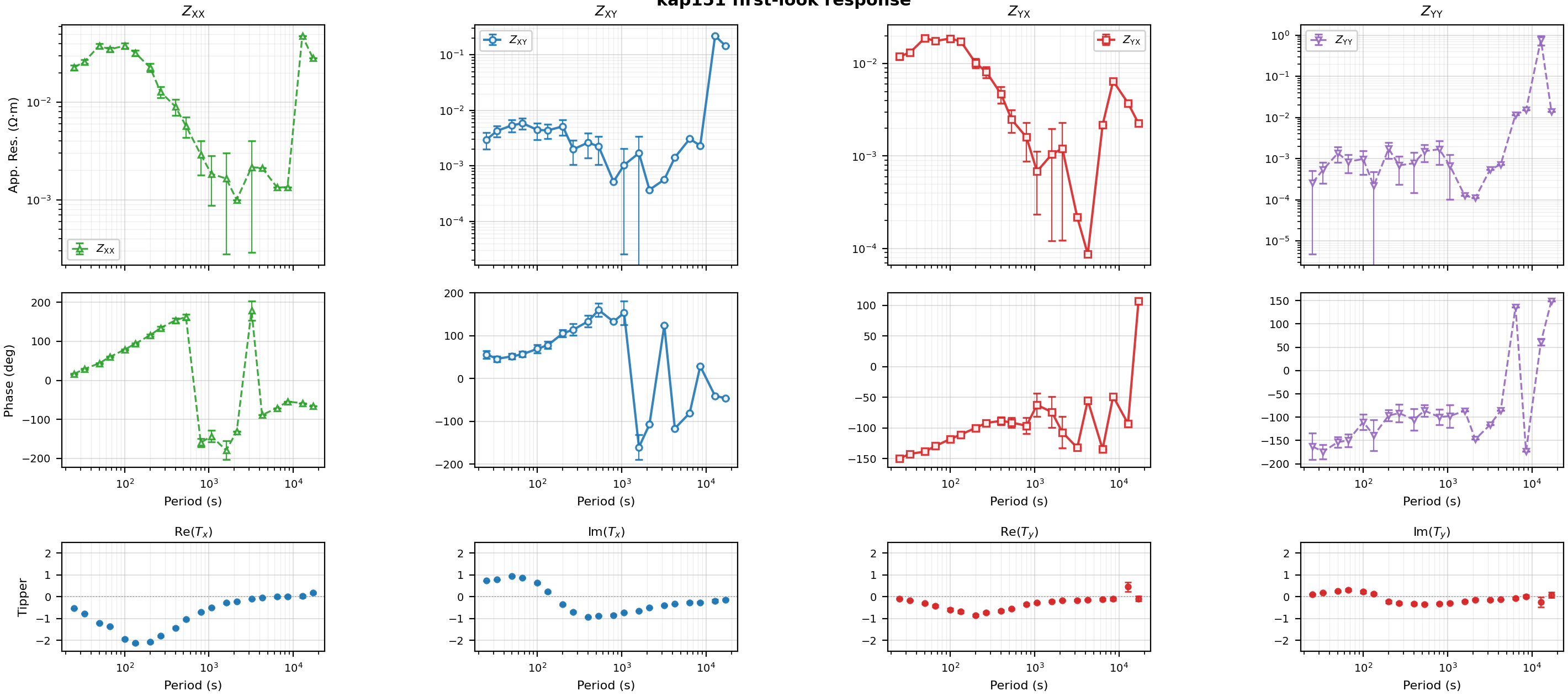
The first row is apparent resistivity on log-log axes. The second row
is phase on a log-period x-axis. The optional third row shows
Re(Tx), Im(Tx), Re(Ty), and Im(Ty). If no tipper exists
or show_tipper=False, the figure uses only the impedance rows.
11.1.16. Overlay A Model Response#
When sites_model is supplied, the station response overlays a
second dataset as dashed curves. If observed and model resistivity are
both available, the function appends an RMS value to component titles.
The RMS is computed in log10(rho) space.
For a component with observed resistivity \(\rho_j^\mathrm{obs}\) and model resistivity \(\rho_j^\mathrm{mod}\) interpolated onto the observed periods, the displayed RMS is
Because the misfit is logarithmic, a factor-of-two error at low resistivity is weighted the same as a factor-of-two error at high resistivity.
>>> from pycsamt.emtools import smooth_mavg
>>> observed = ensure_sites("data/MT/kap03lmt_edis", strict=True)
>>> # For demonstration only: a smoothed copy behaves like a model response.
>>> # In production, pass forward-model or inversion-response EDI data here.
>>> model_like = smooth_mavg(observed, k=5)
>>> fig = plot_station_response(
...     observed,
...     station="kap151",
...     sites_model=model_like,
...     components=("xy", "yx"),
...     period_range=(1e-2, 2e4),
...     show_rms=True,
...     show_tipper=False,
...     figsize=(8.5, 5.2),
...     title="kap151 observed vs model-like response",
... )
>>> fig.savefig("kap151_response_with_model_overlay.png", dpi=200, bbox_inches="tight")
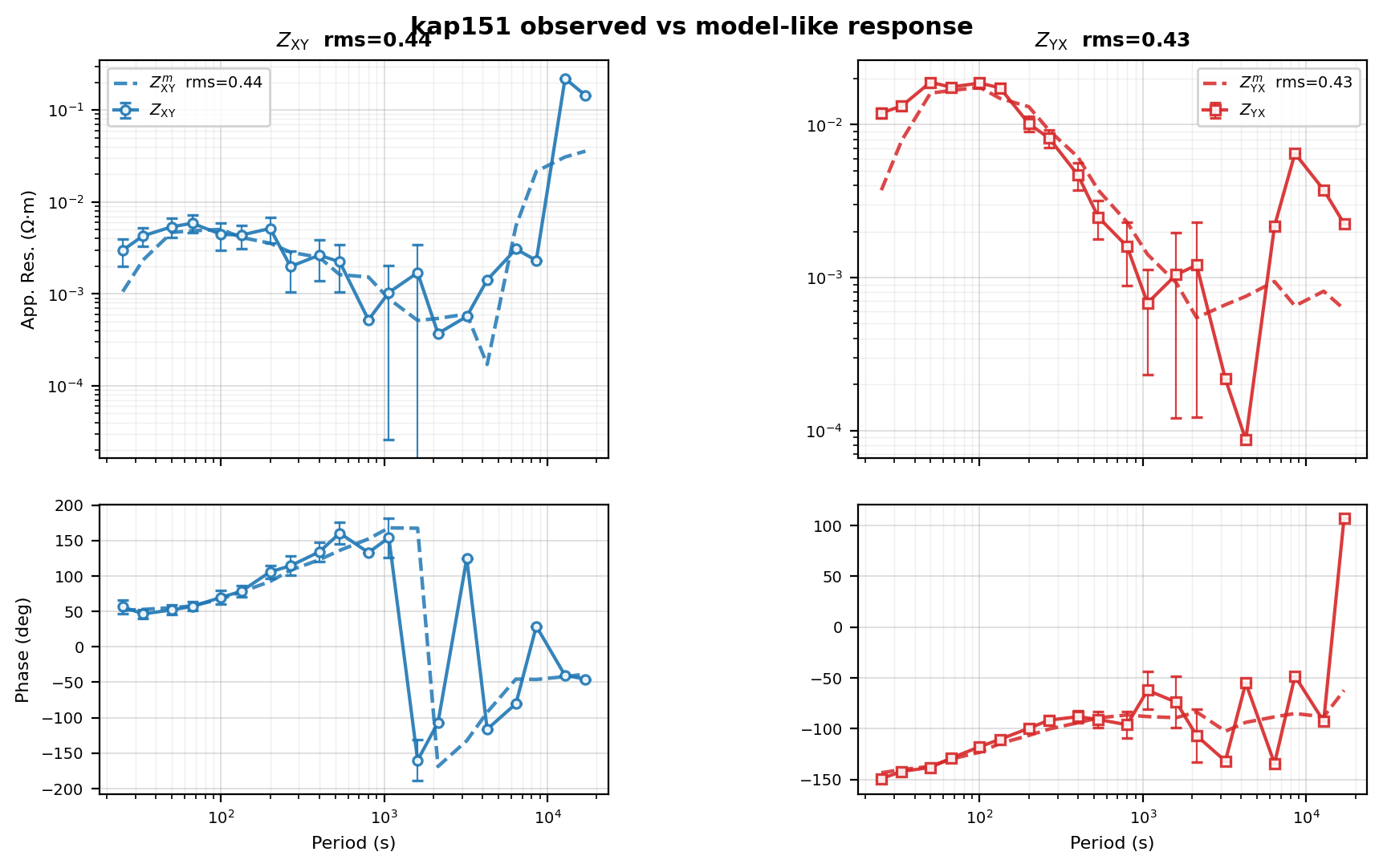
Use this view after inversion or forward modelling to check whether the model misses a whole component, a period band, or only local points. A single RMS number is useful, but the curve shape tells you why the RMS is high or low.
11.1.17. Build A First-Look Report Bundle#
The following script writes a compact first-look bundle for a survey: summary table, missing-section table, frequency coverage, rho/phase curves for a few stations, one pseudo-section, and one station response.
>>> from pathlib import Path
>>> out = Path("inspect_report_l18plt")
>>> out.mkdir(parents=True, exist_ok=True)
>>> survey = ensure_sites("data/AMT/WILLY_DATA/L18PLT", strict=True)
>>> summary = sites_summary(survey, api=False)
>>> summary.to_csv(out / "sites_summary.csv", index=False)
>>> missing = list_missing_sections(survey, require=("mt", "tipper"))
>>> missing_rows = [
...     {"station": station, "missing": ",".join(sections)}
...     for station, sections in missing.items()
... ]
>>> pd.DataFrame(missing_rows).to_csv(out / "missing_sections.csv", index=False)
>>> fig, ax = plt.subplots(figsize=(8.0, 4.5))
>>> _ = plot_coverage(survey, ax=ax)
>>> fig.tight_layout()
>>> fig.savefig(out / "frequency_coverage.png", dpi=200)
>>> subset_names = list(summary["station"].head(4))
>>> subset_paths = [
...     site.edi.path
...     for index, site in enumerate(_iter_items(survey))
...     if _name(site, index) in subset_names
... ]
>>> subset = ensure_sites(subset_paths, strict=True)
>>> ax_rho, ax_phase = plot_rhoa_phi(subset, components=("xy", "yx"))
>>> ax_rho.figure.savefig(out / "rho_phase_subset.png", dpi=200)
>>> fig, ax = plt.subplots(figsize=(10.0, 4.8))
>>> _ = pseudosection(survey, quantity="rho_xy", ax=ax, topo=False)
>>> fig.tight_layout()
>>> fig.savefig(out / "rho_xy_pseudosection.png", dpi=200)
>>> first_station = str(summary["station"].iloc[0])
>>> first_station
'18-001A'
>>> fig = plot_station_response(
...     survey,
...     station=first_station,
...     components=("xy", "yx"),
...     show_tipper=False,
... )
>>> fig.savefig(out / f"station_response_{first_station}.png", dpi=200, bbox_inches="tight")
11.1.18. Reading The Inspection Results#
Treat these outputs as a triage board:
n_freqdiffers between stationsAlign or edit the frequency grid before making survey-wide pseudo-sections or station statistics that assume common samples.
- All stations are missing tipper
Skip tipper diagnostics for that survey. This can be normal for AMT/CSAMT lines.
- Only some stations are missing tipper
Keep those stations out of tipper maps or split the analysis into tipper-capable and impedance-only subsets.
- Rho/phase curves are wildly separated
Check station metadata, static shift, data quality, and whether a few stations dominate the line.
- Pseudo-section anomalies appear only at one frequency
Inspect frequency confidence and errors before interpreting that feature geologically.
- Station response shows diagonal terms comparable to off-diagonals
Follow up with impedance, tensor, dimensionality, and strike tools.
11.1.19. Worked Example#
The gallery example uses the bundled AMT and MT datasets to show the same first-look workflow end to end.
Open the rendered gallery page here: First-look survey inspection (pycsamt.emtools.inspect).