4.5. Map Overlays

Overlay helpers add coordinate transforms, basemaps, contours, labels, profile lines, or terrain to figures assembled by the user. They do not create a second survey model: every visual layer should remain traceable to coordinates and values from the same MapData.

Use pycsamt.map.StationMap or pycsamt.map.MapView for standard maps. The lower-level helpers on this page are useful when a computed value, custom composition, or application callback needs direct control over individual traces.

4.5.1. Coordinates Before Decoration

Web basemaps expect geographic longitude and latitude. Projected field coordinates must therefore be transformed explicitly rather than merely renamed:

>>> import numpy as np
>>> from pycsamt.map import CRSConfig, transform_xy

>>> east = np.array([500000.0, 500250.0])
>>> north = np.array([850000.0, 850200.0])
>>> lon, lat = transform_xy(
...     east,
...     north,
...     crs=CRSConfig(source=32630, target=4326),
... )
>>> np.round(lon, 6).tolist()
[-3.0, -2.997733]
>>> np.round(lat, 6).tolist()
[7.689755, 7.691564]

For station \(i\), the operation is

(1)\[(\lambda_i,\phi_i) =T_{\mathrm{src}\rightarrow4326}(x_i,y_i),\]

where \(T\) includes the source datum and projection. With always_xy=True—the default—arguments remain x, y and WGS84 output remains longitude, latitude even when CRS metadata advertises a different axis order.

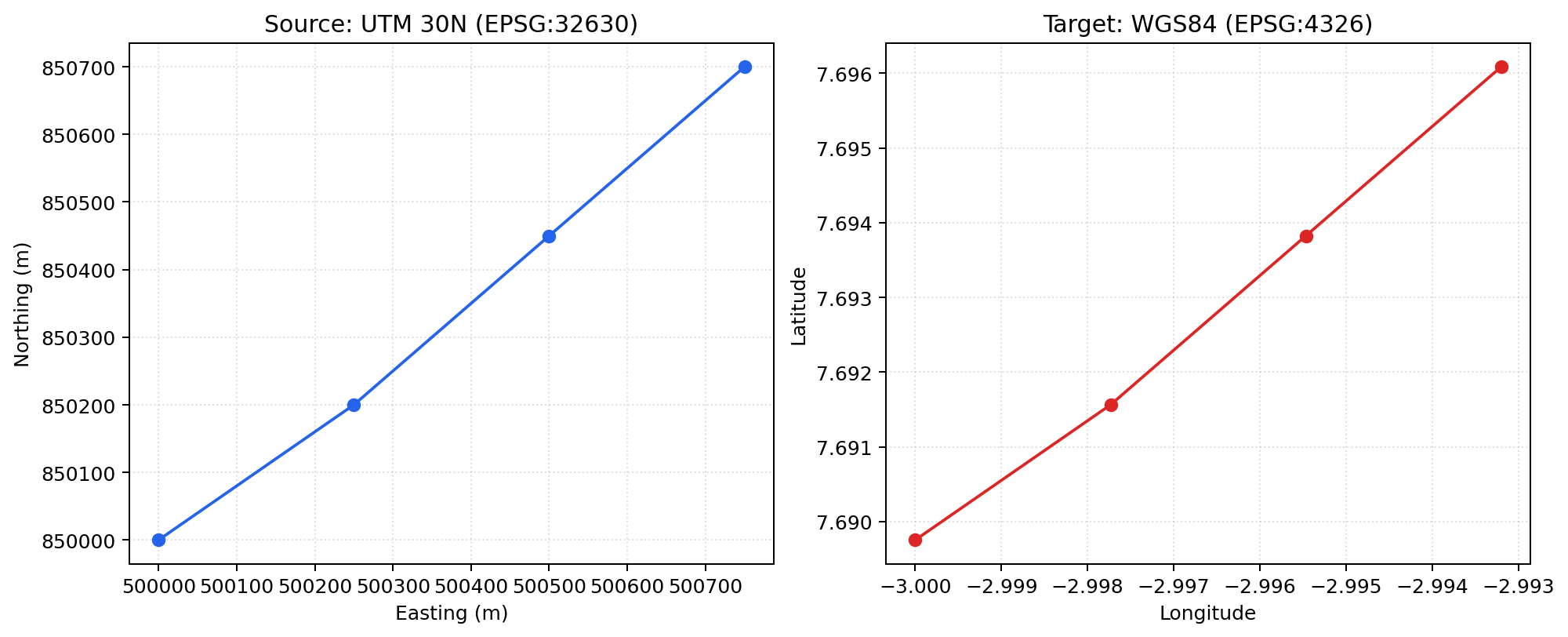
The same four positions in UTM Zone 30N and WGS84. Their numerical scales change completely while their ordering and geometry remain consistent. Plotting the left-hand numbers directly on a geographic basemap would place the survey incorrectly.

pycsamt.map.resolve_crs_info() provides auditable descriptions:

>>> from pycsamt.map import normalize_epsg, resolve_crs_info
>>> normalize_epsg(32630)
'EPSG:32630'
>>> print(resolve_crs_info("utm", zone=30, hemisphere="N"))
EPSG:32630 UTM Zone 30N (WGS 84)

4.5.2. Basemap Extent And Style

pycsamt.map.build_basemap_layout() returns a pycsamt.map.BasemapConfig, not a complete figure:

>>> from pycsamt.map import build_basemap_layout
>>> basemap = build_basemap_layout(lon, lat, bearing=12.0)
>>> print(basemap.style, basemap.zoom, basemap.bearing)
open-street-map 14 12.0
>>> {key: round(value, 6) for key, value in basemap.center.items()}
{'lat': 7.690659, 'lon': -2.998867}

The center is the mean of finite coordinate pairs. Zoom is selected from their largest geographic span and constrained to a practical range. Missing coordinates produce a world view centered at zero. Native token-free styles include open-street-map, carto-positron, and carto-darkmatter; ESRI names such as esri-satellite resolve to a white-bg base plus a raster layer.

4.5.3. Measured Points And Interpolated Surfaces

A contour overlay estimates values between scattered samples. For finite observations \((x_i,y_i,v_i)\) it constructs a regular grid and evaluates

(2)\[\widehat v_{jk}=I(x'_j,y'_k\mid\{x_i,y_i,v_i\}_{i=1}^{n}).\]

The interpolation operator \(I\) is an assumption, not an additional measurement. SciPy supplies linear or requested scattered interpolation when available; the portable fallback assigns the nearest station value.

>>> from pycsamt.map import interpolate_overlay_grid
>>> xi, yi, grid = interpolate_overlay_grid(
...     lon, lat, np.array([100.0, 120.0]), grid_size=12
... )
Traceback (most recent call last):
...
ValueError: At least three finite points are required.

Three points are the mathematical minimum, but rarely provide enough support for geological interpretation.

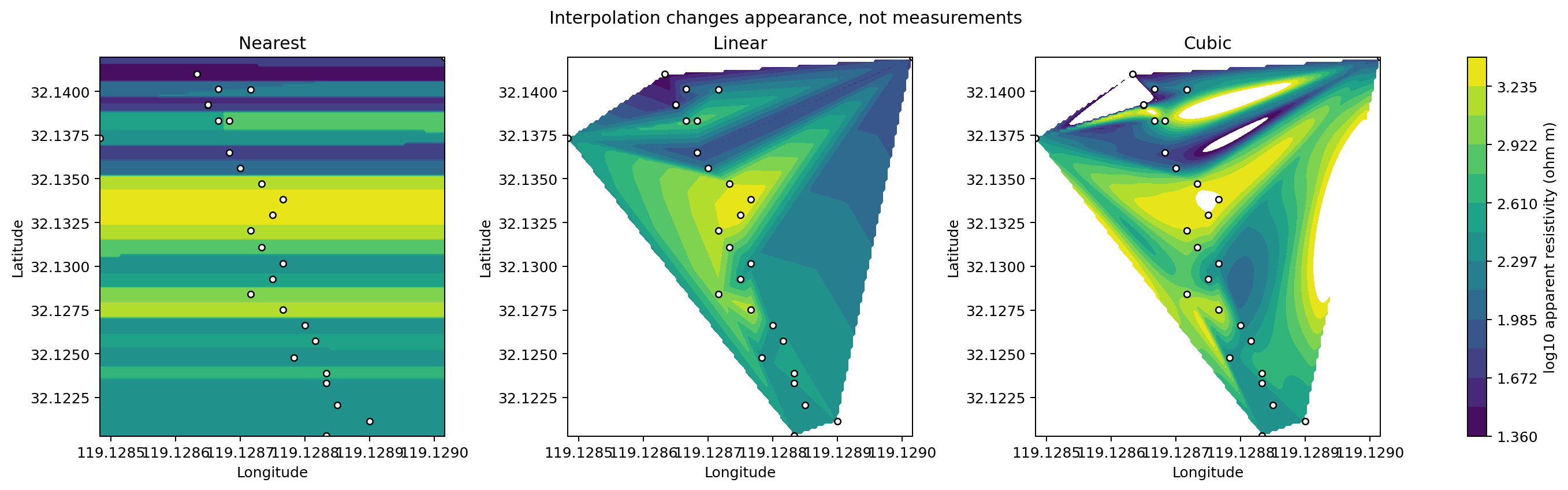
Nearest, linear, and cubic interpolation of the same 28 measured L18 apparent-resistivity values at 102.4 Hz. White markers are the observations. Nearest interpolation is blocky, linear interpolation is piecewise planar, and cubic interpolation introduces smooth extrema; differences away from markers are produced by \(I\), not the EDI files.

Build a Plotly contour trace when the interpolation is appropriate:

>>> from pycsamt.map import build_contour_overlay
>>> contour = build_contour_overlay(
...     np.array([2.0, 2.1, 2.2]),
...     np.array([1.0, 1.1, 1.0]),
...     np.array([100.0, 120.0, 80.0]),
...     levels=8,
...     mode="both",
... )
>>> print(contour.type, len(contour.x), len(contour.y))
contour 80 80

grid_size controls numerical resolution, not information content. Increasing it creates more pixels without creating more field samples.

4.5.4. Lines, Labels, And Response Values

Line and label helpers return either Cartesian Scatter or geographic Scattermap traces according to geo:

>>> from pycsamt.map import (
...     build_profile_line_overlay,
...     build_station_label_overlay,
... )
>>> line = build_profile_line_overlay(lon, lat, geo=True, name="L18")
>>> labels = build_station_label_overlay(
...     lon, lat, ["S00", "S01"], geo=True
... )
>>> print(line.type, labels.type, tuple(labels.text))
scattermap scattermap ('S00', 'S01')

The line follows normalized station order. It communicates acquisition geometry; it does not interpolate the electromagnetic value along the polyline.

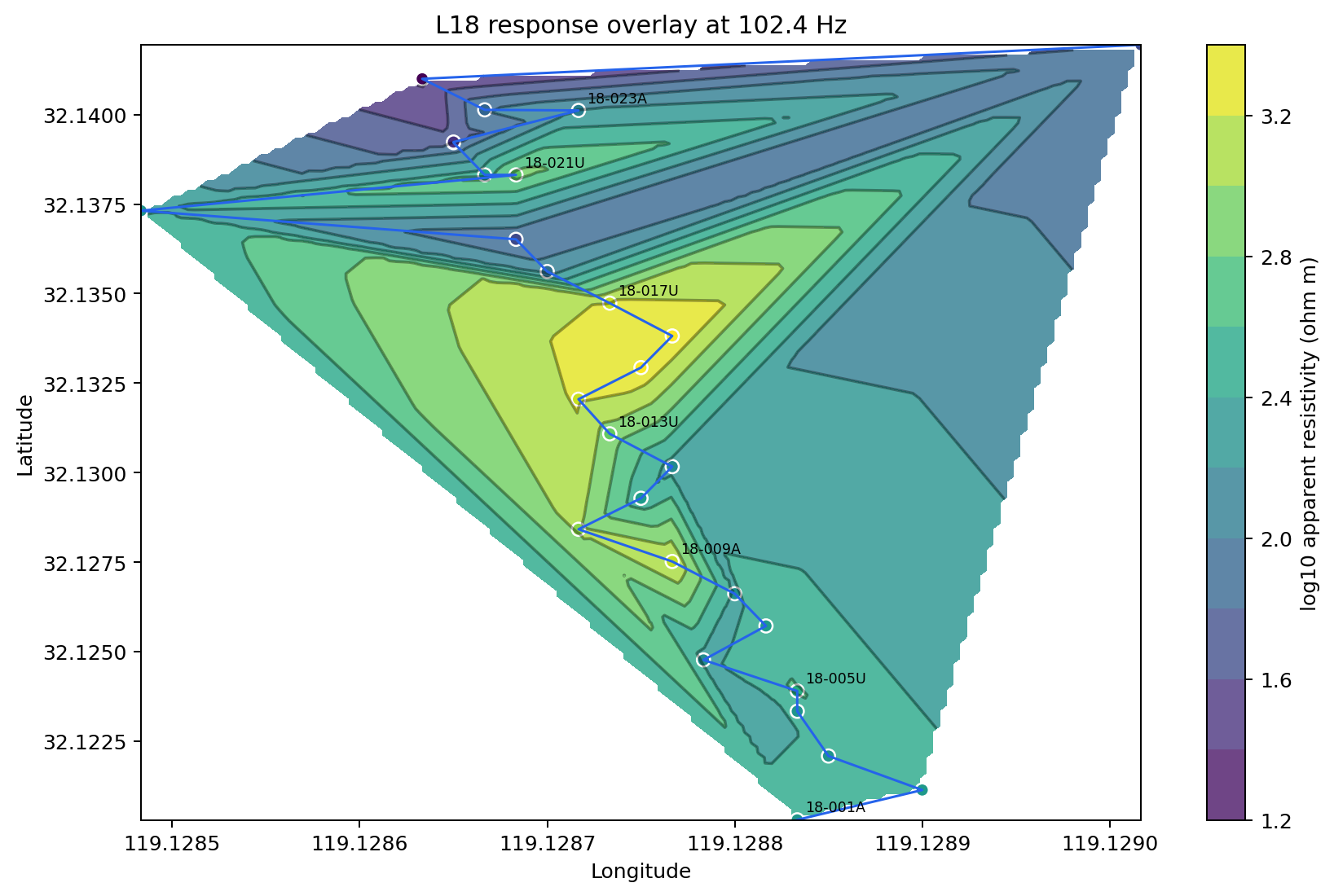
L18 apparent resistivity at the selected 102.4 Hz sample. Measured markers remain visible over the linear contour surface, the blue line shows station order, and only every fourth station is labelled to keep the dense northern turn legible. The large triangular regions near the turn have weak spatial support and should be read cautiously.

4.5.5. Multiple Lines Without Visual Crowding

For a multi-line survey, small multiples often communicate geometry more clearly than 128 labels on one map:

>>> from pycsamt.map import load_lines
>>> data = load_lines("data/AMT/WILLY_DATA", detect="folder")
>>> print(data.lines)
('L18PLT', 'L22PLT', 'L26PLT', 'L30PLT', 'L34PLT')
>>> sum(2 for _profile in data.profiles)
10

Two traces per profile—one line and one label trace—give ten traces. In a combined interactive map, labels can instead be limited to endpoints or exposed through hover text.

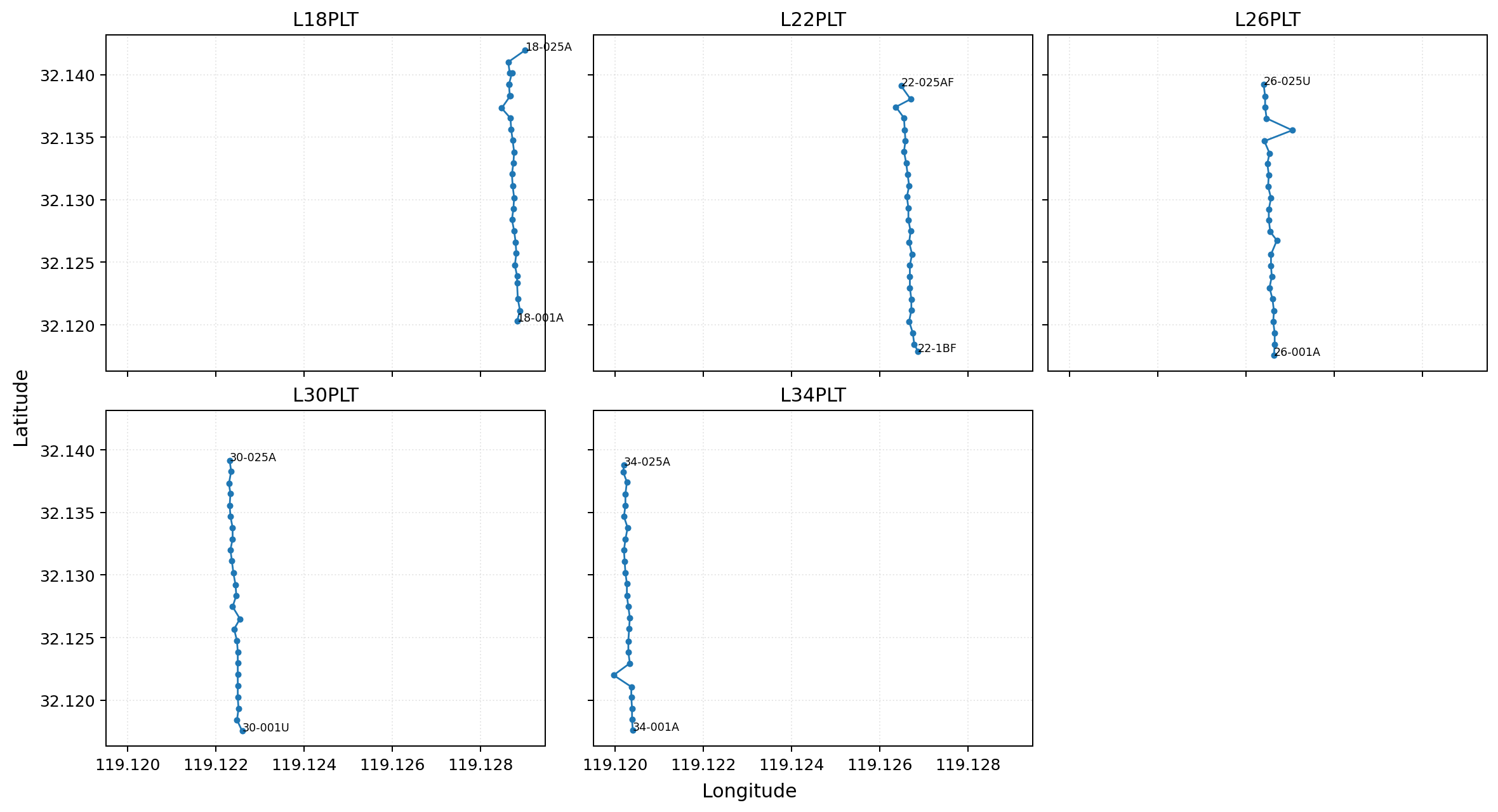
Five profile overlays on identical coordinate limits. Endpoint labels identify acquisition direction without covering every marker, while the grid makes differences in line position and shape directly comparable.

4.5.6. Topography Is Geometry, Not Response

pycsamt.map.build_topography_overlay() returns Mesh3d for scattered elevations and Surface for a two-dimensional grid:

>>> from pycsamt.map import build_topography_overlay
>>> mesh = build_topography_overlay(
...     np.array([0.0, 1.0, 0.0]),
...     np.array([0.0, 0.0, 1.0]),
...     np.array([100.0, 120.0, 110.0]),
...     opacity=0.55,
... )
>>> print(mesh.type, mesh.opacity)
mesh3d 0.55

For scattered stations, vertices are \((x_i,y_i,h_i)\). A mesh connects those supports but does not improve elevation accuracy between them.

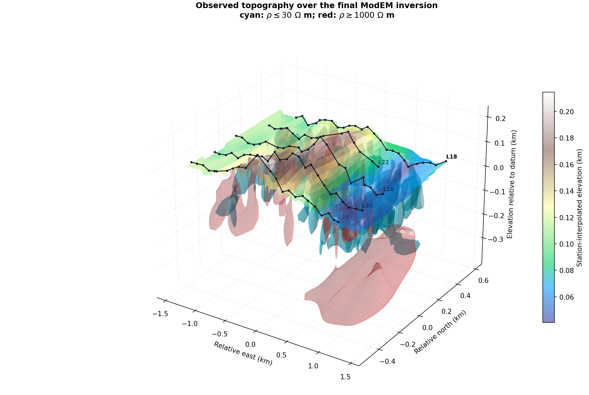
Observed station elevations draped above the final bundled ModEM inversion. Black tracks and points retain the five acquisition lines; the terrain colors show the station-interpolated elevation surface. Below it, cyan marks the 30-ohm-metre conductive boundary and translucent red marks the 1000-ohm-metre resistive boundary. Their relation to relief is now visible without making the terrain opaque or enclosing the model in solid panes.

The terrain is still an overlay rather than an inversion response. Its interpolation is constrained only where stations provide elevations, whereas the two subsurface shells come from the final ModEM resistivity mesh. A spatial coincidence between relief and a shell is therefore an observation to test, not evidence that topography caused or validates the anomaly.

</>View topography-and-ModEM overlay source codeClick to inspect and copy the complete code

def make_modem_topography_overlay() -> None:
    """Drape observed elevations above bodies from the final ModEM model."""
    result, rho, x, y, z = _modem_model()
    edi = load_lines(EDI, detect="folder", recursive=True)
    elevation_by_id = {
        station.id: station.elevation
        for station in edi.stations
        if station.elevation is not None
    }
    modem_data = result.data_obs
    samples = []
    for name, (east, north, _height) in modem_data.site_coords.items():
        short_name = name.split("-", 1)[-1]
        elevation = elevation_by_id.get(short_name)
        if elevation is not None:
            samples.append((name, east / 1000.0, north / 1000.0,
                            elevation / 1000.0))
    names, sx, sy, sh = zip(*samples)
    sx, sy, sh = map(np.asarray, (sx, sy, sh))

    gx = np.linspace(sx.min(), sx.max(), 100)
    gy = np.linspace(sy.min(), sy.max(), 90)
    GX, GY = np.meshgrid(gx, gy)
    GH = griddata((sx, sy), sh, (GX, GY), method="linear")
    nearest = griddata((sx, sy), sh, (GX, GY), method="nearest")
    GH = np.where(np.isfinite(GH), GH, nearest)

    # ModEM nodes are stored from zero; station offsets are centred on the
    # model origin. Shift cell centres into that same coordinate frame.
    mx = (x - 0.5 * (x[0] + x[-1])) / 1000.0
    my = (y - 0.5 * (y[0] + y[-1])) / 1000.0
    xi = np.flatnonzero((mx >= sx.min() - 0.25) & (mx <= sx.max() + 0.25))
    yi = np.flatnonzero((my >= sy.min() - 0.25) & (my <= sy.max() + 0.25))
    zi = np.arange(min(31, len(z)))
    sub = np.log10(rho[np.ix_(zi, yi, xi)])
    spacing = (
        float(np.median(np.diff(z[zi]))) / 1000.0,
        float(np.median(np.diff(my[yi]))),
        float(np.median(np.diff(mx[xi]))),
    )

    fig = plt.figure(figsize=(12.2, 8.2), constrained_layout=True)
    ax = fig.add_subplot(111, projection="3d")
    terrain = ax.plot_surface(
        GX, GY, GH, cmap="terrain", alpha=0.58,
        linewidth=0, antialiased=True, shade=True,
    )
    surface_level = float(np.nanmedian(sh))
    for level, color, alpha in (
        (np.log10(30.0), "#06b6d4", 0.34),
        (np.log10(1000.0), "#dc2626", 0.18),
    ):
        verts, faces, _, _ = marching_cubes(sub, level=level, spacing=spacing)
        ax.plot_trisurf(
            verts[:, 2] + mx[xi[0]],
            verts[:, 1] + my[yi[0]],
            surface_level - verts[:, 0],
            triangles=faces, color=color, alpha=alpha,
            linewidth=0.04, edgecolor=color,
        )

    line_names = np.array([name.split("-")[1] for name in names])
    for line in sorted(set(line_names)):
        keep = line_names == line
        order = np.argsort(sx[keep])
        lx, ly, lh = sx[keep][order], sy[keep][order], sh[keep][order]
        ax.plot(lx, ly, lh + 0.006, color="#111827", linewidth=1.25,
                marker="o", markersize=2.3, zorder=20)
        ax.text(lx[-1], ly[-1], lh[-1] + 0.018, f"L{line}",
                fontsize=8, weight="bold")

    ax.set_title(
        "Observed topography over the final ModEM inversion\n"
        "cyan: $\\rho\leq30$ $\\Omega$ m; red: $\\rho\geq1000$ $\\Omega$ m",
        weight="bold",
    )
    ax.set_xlabel("Relative east (km)")
    ax.set_ylabel("Relative north (km)")
    ax.set_zlabel("Elevation relative to datum (km)")
    ax.view_init(elev=27, azim=-57)
    ax.grid(True, linestyle=":", linewidth=0.6, alpha=0.3)
    for axis in (ax.xaxis, ax.yaxis, ax.zaxis):
        axis.pane.set_alpha(0.0)
        axis._axinfo["grid"].update(
            color=(0.39, 0.45, 0.55, 0.32), linestyle=":", linewidth=0.6,
        )
    cbar = fig.colorbar(terrain, ax=ax, shrink=0.62, pad=0.08)
    cbar.set_label("Station-interpolated elevation (km)")
    fig.savefig(IMAGES / "map_overlays_topography_surface.png", dpi=190)
    plt.close(fig)

4.5.7. Composing A Custom Figure

Overlay helpers return ordinary Plotly objects:

>>> import plotly.graph_objects as go
>>> fig = go.Figure()
>>> fig.add_trace(contour)
Figure({
...
})
>>> fig.update_layout(
...     map=dict(
...         style=basemap.style,
...         center=basemap.center,
...         zoom=basemap.zoom,
...         bearing=basemap.bearing,
...     )
... )
Figure({
...
})

Do not mix Cartesian contour traces with geographic map traces in the same axes. For a geographic filled contour, use the station-map contour_image path described in Station Maps.

4.5.8. Troubleshooting

ImportError during CRS conversion

Install pyproj through the geographic or full dependency extra.

ValueError: At least three finite points are required.

Remove incomplete rows and confirm at least three coordinate/value triples remain. Prefer markers when spatial support is weak.

Contour artifacts cross empty areas

Interpolation operates inside a geometric footprint, not geological boundaries. Retain measured markers, compare interpolation methods, or mask unsupported regions.

Labels overlap

Label endpoints or a regular subset, use hover text for the remainder, or use small multiples as above.

Basemap opens at world scale

No finite longitude/latitude pairs reached the layout helper. Inspect data.has_geo and verify the source CRS.