6.3.20. AI inversion agents

The agents in pycsamt.agents provide task-oriented orchestration around the AI inversion classes in pycsamt.ai.inversion. Each agent can load EDI data, construct model inputs, train or load an inverter, predict resistivity, compute selected diagnostics, create figures, save outputs, and return a standard AgentResult.

Agents do not replace the science API. Use the lower-level inverter classes when you need complete control of datasets, network construction, training loops, loss functions, checkpoints, or research experiments. Use agents when the built-in workflow matches the task and a consistent result contract is valuable.

The figures on this page are executable records of the current agents. The source below reruns the named WILLY sections from the bundled EDI files, so a changed solver, training contract, or plotting path can be reviewed in the same place as its documentation output.

</>View the real-data section regeneration sourceClick to inspect and copy the complete code

def make_agents_real_data_sections(names: set[str] | None = None) -> None:
    """Regenerate legacy-named sections from current WILLY agents."""
    line = PROJECT_ROOT / "data" / "AMT" / "WILLY_data" / "L18PLT"
    sites = ensure_sites(line, recursive=True, verbose=0)
    runs = (
        (
            "agents_ai1d_section.png",
            AIInversionAgent(
                arch="resnet", n_layers=5,
                n_train_samples=10_000, epochs=100,
            ),
            "ai_section",
        ),
        (
            "agents_ensemble_section.png",
            EnsembleAgent(
                n_estimators=5, arch="resnet", n_layers=5,
                n_train_samples=2_000, epochs=30, calibrate=True,
            ),
            "uncertainty_section",
        ),
    )
    for filename, agent, figure_key in runs:
        if names is not None and filename not in names:
            continue
        result = agent.execute({"sites": sites})
        if result.status == "failed":
            raise RuntimeError(f"{filename}: {result.error}")
        figure = result["figures"].get(figure_key)
        if figure is None:
            raise RuntimeError(f"{filename}: missing figure {figure_key!r}")
        _save(figure, filename)
        print(filename, result.summary)

Human review remains required

An agent can coordinate calculations but cannot establish that the training distribution represents the field site, that a predicted model is unique, or that geological interpretation is justified. Non-uniqueness is a property of the inverse problem itself, not something a fast prediction removes. Review input data, training provenance, forward response fit, warnings, uncertainty, and independent evidence before using a result operationally.

6.3.20.1. Agent map

Agent	Main engine	Intended use
pycsamt.agents.AIInversionAgent	pycsamt.ai.inversion.EMInverter1D	Independent layered 1-D prediction at each station, trained from synthetic MT responses or loaded from a checkpoint.
pycsamt.agents.Inv2DAgent	pycsamt.ai.inversion.EMInverter2D	U-Net profile inversion using the complete station–frequency panel to predict a laterally coherent section.
pycsamt.agents.Inv3DAgent	pycsamt.ai.inversion.GCNInverter3D	Graph-based multi-station prediction using coordinates and spatial adjacency, with optional Monte Carlo dropout spread. Training physics is either tiled MT1D or genuine small-grid MT3D; these are not scientifically interchangeable.
pycsamt.agents.EnsembleAgent	pycsamt.ai.inversion.EnsembleInverter	Ensemble inversion, prediction intervals, and optional conformal prediction calibration.
pycsamt.agents.PINNInversionAgent	PINN 1-D, 2-D, or 3-D inverter	Physics-informed inversion without labelled training targets.
pycsamt.agents.ModelZooAgent	Model zoo registry and EMInverter1D	List model metadata, obtain a released checkpoint, or run the zoo prediction shortcut.

Additional agents such as HybridInversionAgent (hybrid inversion), JointInversionAgent, AnomalyDetectionAgent, SensitivityAgent, InversionComparisonAgent, and InversionEvaluationAgent support more specialized review and combination workflows. Start with one primary agent and add these only when the scientific question requires them.

6.3.20.2. Common execution contract

All primary agents use the same call shape:

>>> result = agent.execute({
...     "path": "data/AMT/WILLY_data/L18PLT",
...     "output_dir": "outputs/ai_inversion/L18",
... })

path or sites

Required observed input. path is passed through the canonical pycsamt.emtools._core.ensure_sites() loader. sites accepts an already loaded pycsamt.site.Sites object.

output_dir

Optional output directory for supported checkpoints and figures. If it is omitted, in-memory results can still be returned.

Some agents accept additional execution overrides, such as period_range, coords, adjacency, epochs, or n_train_samples. Constructor parameters remain the clearest way to define a reproducible workflow; runtime overrides should be recorded with the result. A key documented on an agent’s input contract is not automatically wired to internal behaviour — verify a new override changes the result before relying on it operationally.

6.3.20.3. AgentResult

Every execution returns an AgentResult, not a bare array:

>>> if result.status == "failed":
...     raise RuntimeError(
...         f"{result.error}\nSuggested fix: {result.error_fix_hint}"
...     )
>>> print(result.status)
>>> print(result.summary)
>>> print(result.warnings)
>>> print(result.elapsed_seconds)
>>> rms = result.get("rms_global")

The standard fields are:

status

"success", "failed", or "needs_review". A truth test is false only for "failed"; therefore check the exact status when "needs_review" must stop a production workflow.

summary

Short human-readable execution summary.

data

Agent-specific arrays, inverter objects, figures, and paths. Dictionary-like access is available through result["key"] and result.get(...).

warnings

Non-fatal issues. A successful status does not make these optional reading.

error and error_fix_hint

Failure detail and suggested remediation.

llm_interpretation

Optional generated narrative when an API key is configured. This text is commentary, not a validated scientific conclusion.

elapsed_seconds and cost_estimate_usd

Execution duration and estimated LLM cost. Neural-network compute cost is not represented by the LLM cost field.

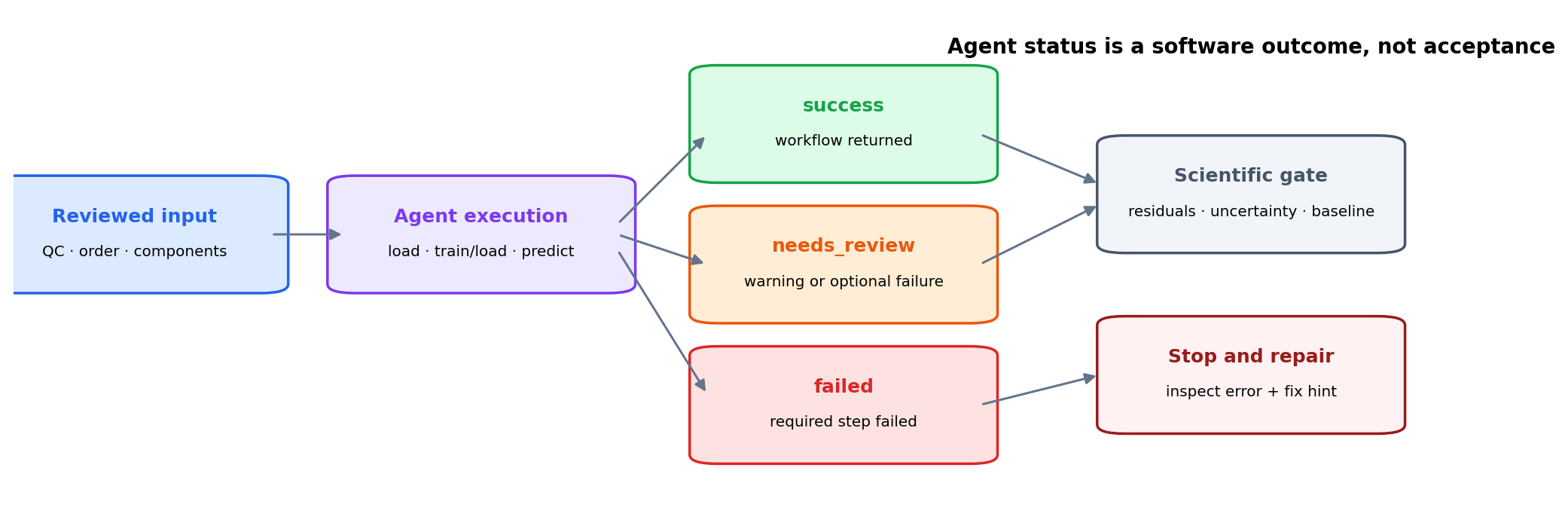
The result status controls software flow. success and needs_review both continue to residual, uncertainty, and baseline checks; failed stops at remediation. None of the three statuses is itself a geological interpretation.

This separation prevents a common automation error. Because bool(result) is true for both success and needs_review, code such as if result: publish(result) is too weak for a controlled release. Test the exact status, then apply an independent scientific decision gate whose thresholds were declared before viewing the preferred inversion.

6.3.20.4. Prepare data before running an agent

Load and inspect the same data independently before delegating inversion. The survey used throughout this page is the bundled Willy AMT line:

>>> from pycsamt.emtools._core import ensure_sites
>>> sites = ensure_sites(
...     "data/AMT/WILLY_data/L18PLT",
...     recursive=True,
...     verbose=0,
... )
>>> print("Usable stations:", len(sites))
Usable stations: 28

Review quality control, impedance components, frequencies, coordinates, dimensionality, static shift, and processing provenance first. The 1-D agent includes an important fast-fail guard: it verifies that at least one station can produce a finite impedance feature vector before spending time generating synthetic data and training. This guard catches empty or corrupted inputs, but it is not a complete QC assessment.

6.3.20.5. Deep-learning backend

The inversion agents lazily require PyTorch or TensorFlow. If neither backend is available, they return a failed AgentResult with an installation hint instead of failing package import:

>>> from pycsamt.backends import get_backend, list_backends
>>> print(get_backend())
torch
>>> print(list_backends())
{'torch': True, 'tensorflow': True}

Verify the project environment before a long run. Also record backend name, version, hardware, random seeds where exposed, and numerical precision. Results can differ across backends and devices even when high-level parameters match — the runs captured on this page used a CPU-only PyTorch 2.5 build, so timings will differ on GPU or TensorFlow.

6.3.20.6. Read every inversion as a contract

An agent-generated section is meaningful only when its axes and transformations are explicit. Throughout the newly generated figures in this guide, stations are columns labelled along the top. Frequency panels place high frequency at the top and low frequency at the bottom; model panels place shallow depth or the first layer at the top. Keep this convention when saving custom figures so the visual direction does not reverse between data and model space.

Before interpreting color, establish five facts:

• whether the vertical coordinate is layer index, depth below station, or absolute elevation;

• how thickness predictions were converted to interfaces or a common grid;

• whether the color represents \(\log_{10}\rho\), linear resistivity, residual, or standard deviation;

• whether compared panels share limits and masks;

• which response-space diagnostic accompanies the section.

A few archived agent figures on this page still use a Bostick-derived display depth based on the agent’s very broad default \(10^{-4}\)–\(10^3\) Hz training grid. Their axes can extend to hundreds or thousands of kilometres. That plotting scale is neither the WILLY depth of investigation nor permission to interpret deep structure — it is a reminder that the class default was never chosen for this survey. The Inv3DAgent examples below instead build the frequency grid from the loaded stations, which is the same fix worth applying anywhere a sub-2-km target is expected: rerun with a reviewed AMT frequency contract, reconstruct physical layered responses, and clip only the display after preserving the complete model array. See AI inversion concepts for the distinction between configured depth, skin-depth scale, and defensible interpretation depth.

6.3.20.7. AIInversionAgent: 1-D workflow

pycsamt.agents.AIInversionAgent performs this built-in sequence:

1. load observed stations;

2. interpolate impedance-derived features onto a common frequency grid;

3. generate synthetic layered MT training examples unless a checkpoint loads;

4. fit EMInverter1D;

5. predict layer resistivities and thicknesses for each usable station;

6. forward-model each prediction and calculate a log-resistivity RMS where possible;

7. create convergence and section figures;

8. optionally save the inverter and figures.

Train from synthetic data

>>> from pycsamt.agents import AIInversionAgent
>>> agent = AIInversionAgent(
...     arch="resnet",
...     n_layers=5,
...     n_train_samples=10_000,
...     epochs=100,
... )
>>> result = agent.execute({
...     "sites": sites,
...     "output_dir": "outputs/ai_inversion/L18_1d",
... })
>>> print(result.status, result.summary)
success AI inversion (resnet, 5 layers): 28 stations predicted. RMS 1.135. 2 figure(s).

Supported architecture names are "resnet", "cnn1d", and "fcn". The default workflow uses 40 log-spaced frequencies from \(10^{-4}\) to \(10^3\) Hz, 2,000 synthetic examples, five layers, and 30 epochs. Those defaults are convenient workflow settings, not evidence of production adequacy: running the same survey with the constructor defaults instead of the values above still completes in about a minute, but the fitted network only reaches RMS ≈ 3.9 — more than three times the 10,000-sample, 100-epoch run captured above, which took about fourteen minutes on a single CPU core. Sample count and epoch budget are part of the scientific configuration, not incidental performance knobs.

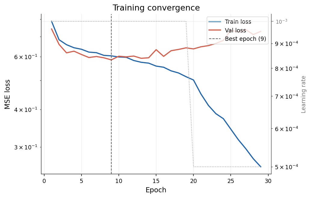
Requesting 100 epochs did not mean training ran for 100 epochs: validation loss stopped improving at epoch 9 and patience-based early stopping ended the run at epoch 29, after the learning-rate scheduler had already cut the rate once. Train loss kept falling past that point while validation loss drifted back up — a plain overfitting signature that the epoch count alone would not have shown.

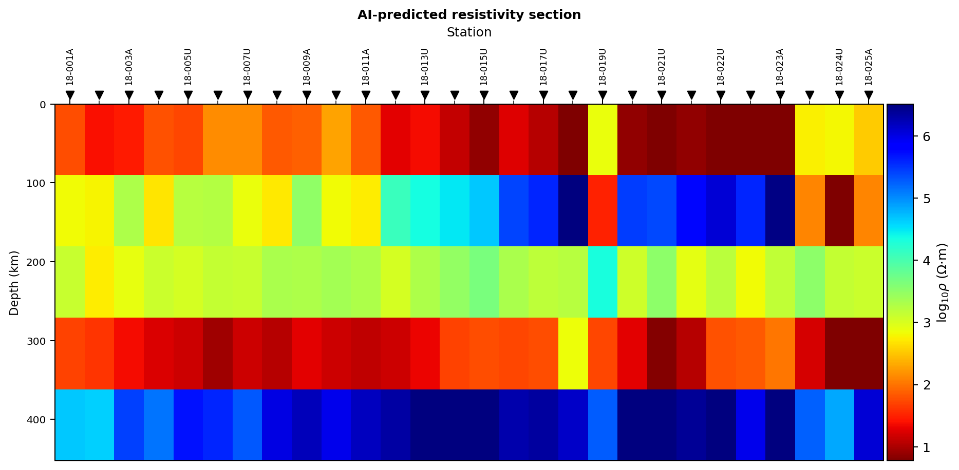
Each column is one station’s independently predicted layered model; there is no lateral continuity constraint between neighbours here, which is the gap Inv2DAgent and Inv3DAgent are built to close.

The regenerated section also exposes a physically implausible cumulative depth exceeding 450 km. That scale comes from unconstrained predicted layer thicknesses; the improved response RMS does not rescue it. Treat this run as a rejected field model and constrain thickness/depth priors before retraining.

The generated training set currently uses the MT 1-D solver, 3% noise, seed 42, and one generation job. If a project requires different priors, correlated noise, missing-data patterns, other solvers, or explicit train/validation/test control, use pycsamt.ai.inversion.EMInverter1D directly as documented in AI inversion data preparation and Training AI inversion models.

Run from a local checkpoint

>>> agent = AIInversionAgent(
...     pretrained="outputs/ai_inversion/L18_1d_quick/ai_inverter_resnet.pkl.npz",
... )
>>> result = agent.execute({"sites": sites})
>>> print(result.status, result.summary, round(result.elapsed_seconds, 1))
success AI inversion (resnet, 5 layers): 28 stations predicted. RMS 3.900. 1 figure(s). 7.1

Loading the earlier, faster checkpoint (2,000 samples, 30 epochs) reproduces its RMS 3.9 fit in about seven seconds instead of retraining — the whole cost of the workflow moves from training to a single forward pass per station. If checkpoint loading fails, the agent adds a warning and falls back to fresh training. Inspect warnings so an expensive fallback is not mistaken for use of the approved checkpoint.

Inspect 1-D outputs

>>> predictions = result["predictions"]
>>> rms_per_station = result["rms_per_station"]
>>> rms_global = result["rms_global"]
>>> first_model = result["best_model"]
>>> len(predictions), list(predictions)[:3]
(28, ['18-001A', '18-002U', '18-003A'])
>>> predictions["18-001A"]
array([0.75388265, 3.24265292, 2.29955796, 2.2847247 , 4.22003814])
>>> first_model["station"], [round(r, 1) for r in first_model["resistivity"]]
('18-001A', [5.7, 1748.4, 199.3, 192.6, 16597.3])

predictions maps station names to log10 resistivity arrays. The best_model label means the first successfully predicted station in the current implementation; it is not selected as the statistically best station. It contains linear resistivity and thickness arrays plus log resistivity.

The forward RMS compares each station’s observed log10 apparent resistivity against the forward response of its own predicted model, interpolated onto the same periods:

(1)\[\mathrm{RMS}_s = \sqrt{\frac{1}{N_s}\sum_{i=1}^{N_s} \Bigl(\log_{10}\rho_{a,i}^{\mathrm{obs}} - \log_{10}\rho_{a,i}^{\mathrm{pred}}\Bigr)^2}\]

with \(N_s\) the number of finite, overlapping periods at station \(s\), and rms_global the mean of \(\mathrm{RMS}_s\) over stations. It is useful as a response-fit diagnostic, matching the more general RMS misfit idea, but unlike a fully weighted misfit it is not normalised by measurement error, so it is not a complete impedance likelihood, phase fit, or proof of geological correctness.

Executed small-run audit

The documentation generator also runs a compact CPU example rather than asking readers to infer behavior from the longer historical runs above. It uses AIInversionAgent(arch="fcn", n_layers=5, n_train_samples=240, epochs=12) on all 28 WILLY L18 stations. The call returns success and produces two figures, but repeated executions can differ because the agent does not expose every backend determinism control. Preserve the actual history and arrays from each run rather than copying one displayed RMS into a new report.

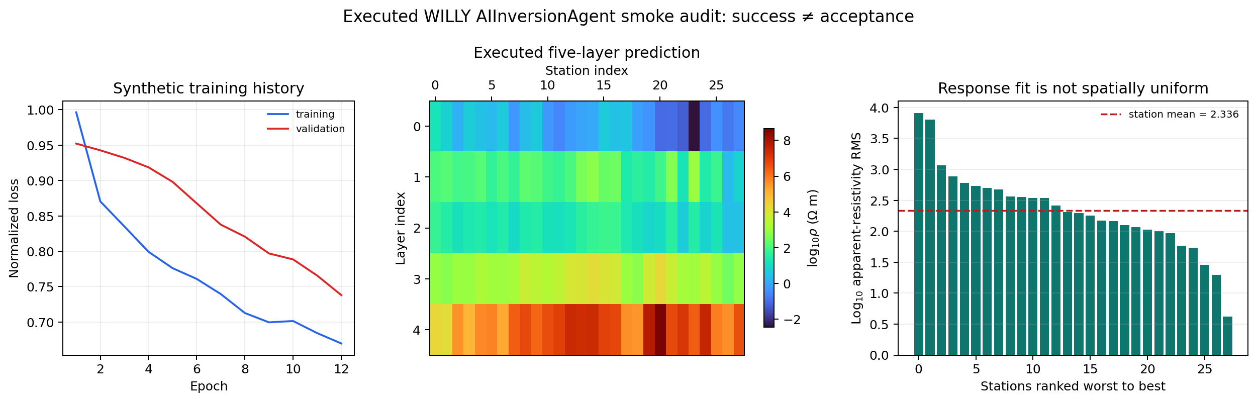
Executed small-run audit. Stations are columns labelled at the top of the inversion panel. The response panel ranks the same stations by the metric in (1); its dashed line is the station mean, not an acceptance threshold.

The section is visually structured, yet the station RMS values span a wide range and some predicted log-resistivities approach implausibly extreme values. The appropriate outcome is therefore workflow success, scientific review required. Increasing training budget may help, but the next action is not automatically “train longer”: first compare the synthetic resistivity and thickness priors with field response support, inspect the worst stations by frequency and phase, and reconstruct responses from the physical layered models. This is why an inversion plot and its response audit belong together.

Compare CNN1D, ResNet, and FCN under one contract

AIInversionAgent exposes three 1-D architecture names. They receive the same flattened response contract and predict the same layered target, but they encode different assumptions:

cnn1d

Convolutions scan neighbouring feature positions with shared kernels. This can learn local frequency-pattern motifs efficiently, but only when the feature ordering keeps physically neighbouring frequencies together. A block layout that concatenates all resistivities and then all phases creates a boundary where convolutional locality changes meaning.

resnet

Residual blocks learn corrections around identity paths. Skip connections generally make deeper networks easier to optimize, but they do not prevent overfitting, domain shift, or an unsuitable synthetic prior. Validation behavior still decides whether the added capacity helped.

fcn

A fully connected network lets every input feature interact immediately with every hidden unit. It does not encode frequency locality, but its simpler inductive structure can be competitive for a small tabular-style response vector and a modest training budget.

A matched smoke-test loop is:

>>> from pycsamt.agents import AIInversionAgent
>>> architecture_results = {}
>>> for architecture in ("cnn1d", "resnet", "fcn"):
...     result = AIInversionAgent(
...         arch=architecture,
...         n_layers=5,
...         n_train_samples=240,
...         epochs=12,
...     ).execute({"sites": sites})
...     architecture_results[architecture] = result
...     print(
...         architecture,
...         result.status,
...         round(result["rms_global"], 3),
...     )
cnn1d success 2.008
resnet success 1.094
fcn success 1.052

These are captured values for the generated figure, not stable package benchmarks. The high-level agent fixes the synthetic generator seed but does not expose every backend determinism setting, so rerunning may change the numbers. A publishable architecture study must reuse an explicitly persisted train/validation/test dataset, match preprocessing and target transforms, report parameter counts and compute, and repeat each architecture over several training seeds.

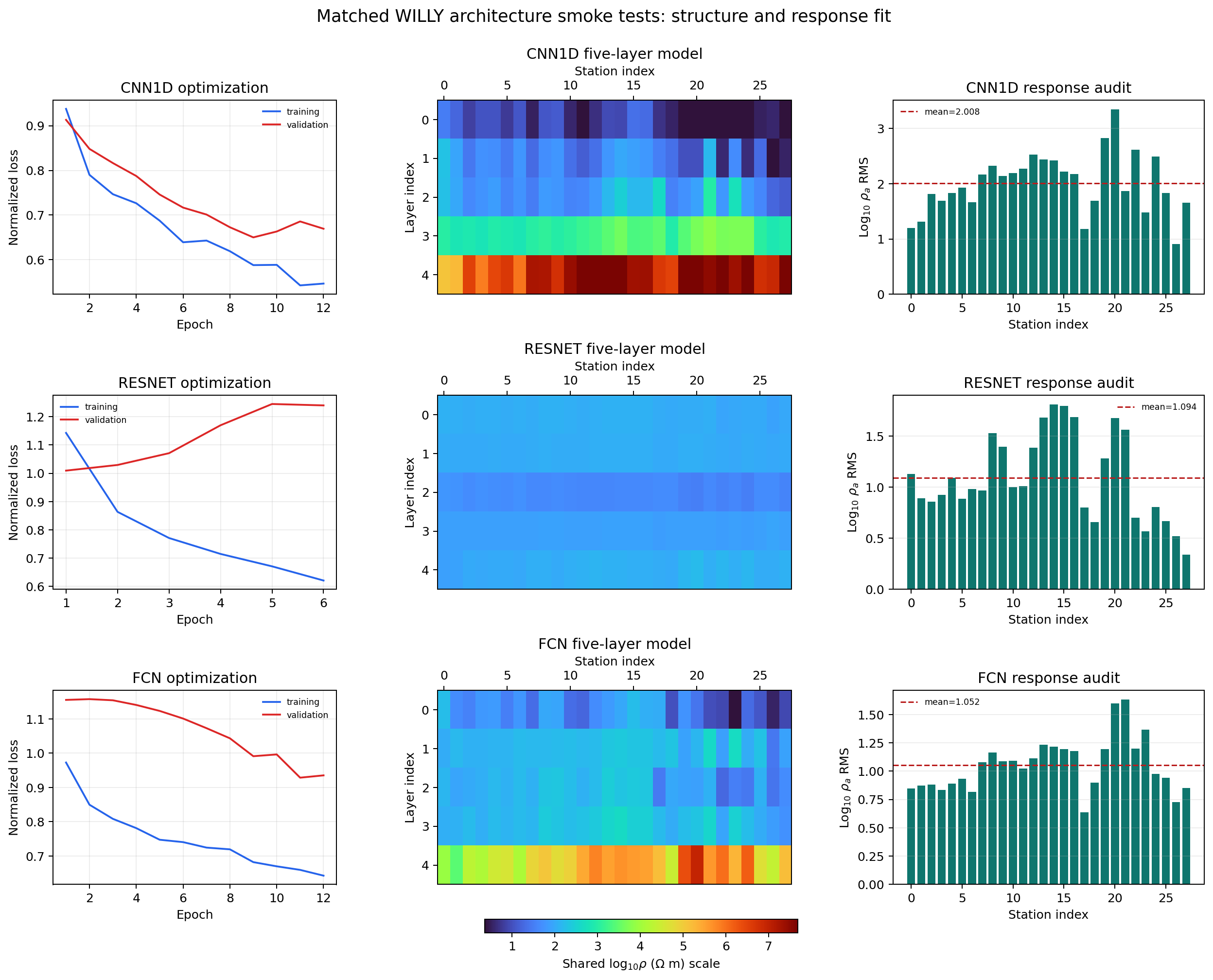
Executed architecture comparison. Every row uses the same sample, layer, station, and epoch budget. Stations are columns at the top of each model; all three model panels share one color scale, and each response panel shows its station-mean RMS as a dashed line.

In this captured run, CNN1D’s validation loss decreases but stays well above training loss, its mean RMS is highest, and the shared scale exposes extreme values in its deepest layer. That combination suggests under-supported target amplitudes rather than a trustworthy deep conductor or resistor. ResNet lowers the response RMS substantially, yet its validation curve becomes unstable and finishes by rising sharply; accepting it solely because its RMS beats CNN1D would ignore an overfitting warning. FCN has the lowest mean RMS and the most orderly validation descent here, although several stations remain much worse than the mean and its deep-layer amplitudes are still broad.

The correct conclusion is conditional: FCN is the best small-budget candidate for the next controlled experiment, not the best WILLY inverter. Repeated-seed holdout error, phase residuals, response reconstruction, model bounds, depth stability, and comparison with classical inversion can reverse the ordering. Also compare station-by-station patterns: if all architectures fail at the same stations, data quality or domain mismatch is more plausible than an architecture-specific problem.

6.3.20.8. Inv2DAgent: profile workflow

pycsamt.agents.Inv2DAgent assembles a station–frequency input panel, trains a U-Net-style inverter, and predicts the complete profile at once. Its physics argument now separates two scientifically different training contracts. The default "mt1d" path tiles independent layered responses into profile-shaped examples; it is a pseudo-2-D training model, not a 2-D electromagnetic simulation. The "mt2d" path draws laterally correlated resistivity fields and computes their TE responses with the 2-D Maxwell training model. Choosing between them changes the training distribution and forward physics, not merely runtime.

The lightweight, tiled path remains useful for smoke tests and is the path used by the captured WILLY example below:

>>> import numpy as np
>>> from pycsamt.agents import Inv2DAgent
>>> from pycsamt.ai.inversion import sites_to_features_1d
>>> from pycsamt.emtools import frequency_for_depth
>>> dense, measured_frequency, _ = sites_to_features_1d(
...     sites, comp="xy", n_freqs=64,
... )
>>> rho_reference = float(
...     10.0 ** np.nanmedian(dense[:, :measured_frequency.size])
... )
>>> frequency_min = max(
...     float(measured_frequency.min()),
...     float(frequency_for_depth(2000.0, rho_reference)),
... )
>>> _, frequency, _ = sites_to_features_1d(
...     sites, comp="xy", n_freqs=24,
...     freq_min=frequency_min,
...     freq_max=float(measured_frequency.max()),
... )
>>> agent = Inv2DAgent(
...     n_depth=40,
...     freqs=frequency,
...     depth_max=2000.0,
...     n_components=2,
...     arch="unet",
...     n_train_profiles=500,
...     n_stations_per_profile=10,
...     epochs=80,
...     physics="mt1d",
... )
>>> result = agent.execute({
...     "sites": sites,
...     "output_dir": "outputs/ai_inversion/L18_2d",
...     "topography": True,
... })
>>> print(result.status, result.summary)
success 2-D AI inversion (U-Net): 10 stations x 40 depth cells. RMS=1.780. 2 figures.

n_components is 2 by default — log10 apparent resistivity and phase for the xy component, matching what generate_dataset() actually produces. It is not four Re/Im tensor channels; keep it at 2 unless a custom data pipeline supplies a genuinely wider panel. The frequency and depth parameters are explicit for the same reason as in the graph example below: leaving the legacy \(10^{-4}\) Hz default in an AMT example would create a hundreds-of-kilometres display grid unrelated to the WILLY target. depth_max controls the output parameterization, not verified depth of investigation.

For a physics-coupled training set, request the 2-D Maxwell path explicitly:

>>> maxwell_agent = Inv2DAgent(
...     n_depth=24,
...     freqs=frequency,
...     depth_max=2000.0,
...     n_train_profiles=100,
...     n_stations_per_profile=10,
...     epochs=80,
...     physics="mt2d",
...     station_spacing_m=125.0,
...     correlation_length_x_m=(250.0, 1000.0),
...     correlation_length_z_m=(75.0, 350.0),
...     lambda_x=1e-3,
...     lambda_z=5e-4,
...     lambda_tv=1e-4,
... )
>>> print(maxwell_agent.physics, maxwell_agent.n_depth)
mt2d 24

This constructor example is intentionally non-executing beyond configuration: a hundred finite-difference realizations are a real training workload, not a documentation smoke test. During execute, each realization uses a regular synthetic grid with n_stations_per_profile columns, n_depth cells, and the declared station_spacing_m. The field survey’s irregular coordinates are not used to generate those synthetic models. Correlation-length ranges, the log-resistivity mean and spread, mesh limits, frequency grid, and depth must therefore be recorded as training provenance.

Inv2DAgent(physics="mt2d") itself always reads its observed panel from a real Sites collection, even though its training distribution is fully synthetic – so it cannot demonstrate a survey-free workflow on its own. The science API underneath it can: EMInverter2D trained directly on generate_2d_maxwell_dataset() output, then evaluated against a hand-built target forward-modelled with the same MT2DAdapter, needs no field data anywhere in the loop:

</>View the fully synthetic EMInverter2D demo sourceClick to inspect and copy the complete code

def make_agents_inv2d_synthetic_demo() -> None:
    """EMInverter2D on a fully synthetic target -- no real survey involved.

    Unlike the WILLY examples above, nothing here is constrained by a real
    line's station count, frequency band, or wall-clock budget: the "true"
    model is a hand-built, smoothed compact conductor (matched to the
    training distribution's own correlation length so it is not an
    out-of-distribution shape), forward-modelled with the same
    :class:`~pycsamt.forward.maxwell.mt2d.MT2DAdapter` the training data
    generator uses internally, then inverted by a freshly trained
    :class:`~pycsamt.ai.inversion.inv2d.EMInverter2D`. This is the
    EMInverter2D/Maxwell2DDatasetConfig science-API layer beneath
    ``Inv2DAgent(physics="mt2d")``, not a captured ``Inv2DAgent.execute()``
    result -- ``Inv2DAgent`` always reads its observed panel from a real
    ``Sites`` collection, even on the synthetic-training ``"mt2d"`` path.
    """
    from scipy.ndimage import gaussian_filter

    from pycsamt.ai.geology import GeologyGrid
    from pycsamt.ai.inversion.inv2d import EMInverter2D
    from pycsamt.ai.training.dataset2d import _solver_mesh_and_conductivity
    from pycsamt.api.mesh import PYCSAMT_MESH

    try:
        import torch

        torch.manual_seed(7)
    except ImportError:
        pass
    np.random.seed(7)

    n_sta, n_depth = 24, 24
    dx_m, depth_max_m = 100.0, 1200.0
    grid = GeologyGrid.regular_2d(
        nx=n_sta, nz=n_depth, dx_m=dx_m, dz_m=depth_max_m / n_depth
    )
    freqs = np.geomspace(2.0, 400.0, 12)

    # Hand-built true model: a background with a compact conductor blob,
    # Gaussian-smoothed so its spatial scale matches the correlation
    # lengths below rather than presenting the network with a sharp box
    # it never saw an analogue of during training.
    log_true_rho = np.full((n_depth, n_sta), 2.0)  # log10(100 ohm.m)
    z_core = slice(int(n_depth * 0.35), int(n_depth * 0.65))
    x_core = slice(int(n_sta * 0.35), int(n_sta * 0.65))
    log_true_rho[z_core, x_core] = np.log10(5.0)  # 5 ohm.m core
    log_true_rho = gaussian_filter(log_true_rho, sigma=(1.8, 1.8))
    true_rho = 10.0**log_true_rho

    mesh_true, conductivity_true = _solver_mesh_and_conductivity(
        grid, true_rho, freqs, safety_factor=6.0, max_mesh_cells=20_000
    )
    receivers = ReceiverSet(
        [[float(x), 0.0] for x in grid.x_m],
        [f"S{i:02d}" for i in range(n_sta)],
    )
    true_problem = MaxwellProblem(
        mesh_true, conductivity_true, freqs, receivers, components=("zxy",)
    )
    true_result = MT2DAdapter().solve(true_problem)
    if not true_result.success:
        raise RuntimeError("synthetic true-model forward solve failed.")
    true_survey = SurveyData(
        impedance=true_result.impedance_v_a,
        frequencies_hz=true_result.frequencies_hz,
        station_names=true_result.receiver_names,
        components=true_result.components,
        coordinates_m=[[float(x), 0.0, 0.0] for x in grid.x_m],
        valid=true_result.valid,
    )

    mu0 = 4.0e-7 * np.pi

    def _samples_to_arrays(samples):
        n_freq = len(freqs)
        X = np.empty((len(samples), 2, n_freq, n_sta), dtype=np.float32)
        y = np.empty((len(samples), n_depth, n_sta), dtype=np.float32)
        for i, sample in enumerate(samples):
            zxy = sample.survey.impedance[:, :, 0]
            f = sample.survey.frequencies_hz[None, :]
            rho_a = np.abs(zxy) ** 2 / (2.0 * np.pi * f * mu0)
            phase = np.degrees(np.angle(zxy))
            X[i, 0] = np.log10(np.clip(rho_a, 1e-12, None)).T
            X[i, 1] = phase.T
            y[i] = np.log10(sample.resistivity_ohm_m)
        return X, y

    def _survey_to_x(survey):
        zxy = survey.impedance[:, :, 0]
        f = survey.frequencies_hz[None, :]
        rho_a = np.abs(zxy) ** 2 / (2.0 * np.pi * f * mu0)
        phase = np.degrees(np.angle(zxy))
        x = np.empty((1, 2, len(freqs), n_sta), dtype=np.float32)
        x[0, 0] = np.log10(np.clip(rho_a, 1e-12, None)).T
        x[0, 1] = phase.T
        return x

    config = Maxwell2DDatasetConfig(
        dataset_id="agents-inv2d-synthetic-demo",
        grid=grid,
        correlation_length_x_m=(300.0, 900.0),
        correlation_length_z_m=(100.0, 300.0),
        frequencies_hz=freqs,
        station_x_m=grid.x_m,
        n_realizations=100,
        seed=0,
        log_resistivity_mean=2.0,
        log_resistivity_std=0.4,
        components=("zxy",),
        mesh_safety_factor=4.0,
        max_mesh_cells=20_000,
    )
    dataset = generate_2d_maxwell_dataset(config)
    X_train, y_train = _samples_to_arrays(dataset.select("train"))

    inverter = EMInverter2D(
        n_components=2, n_depth=n_depth, n_stations=n_sta, n_freqs=len(freqs)
    )
    inverter.fit(X_train, y_train, epochs=80, patience=15, verbose=False, seed=7)
    history = inverter._history

    X_true = _survey_to_x(true_survey)
    log_pred = inverter.predict(X_true)[0]
    log_true = np.log10(true_rho)
    rmse = float(np.sqrt(np.nanmean((log_pred - log_true) ** 2)))
    print(
        "agents_inv2d_synthetic_demo.png",
        f"n_train={len(dataset.select('train'))}",
        f"epochs_run={len(history['train_loss'])}",
        f"rmse={rmse:.3f}",
    )

    fig = plot_inversion_result_2d(
        log_pred,
        log_true=log_true,
        depths=None,
        stations=grid.x_m / 1000.0,
        depth_max=depth_max_m,
        show_mesh=True,
        mesh_style=PYCSAMT_MESH.style_for("review"),
        train_loss=np.array(history["train_loss"]),
        val_loss=np.array(history["val_loss"]),
        suptitle="EMInverter2D on a fully synthetic target",
    )
    _save(fig, "agents_inv2d_synthetic_demo.png")

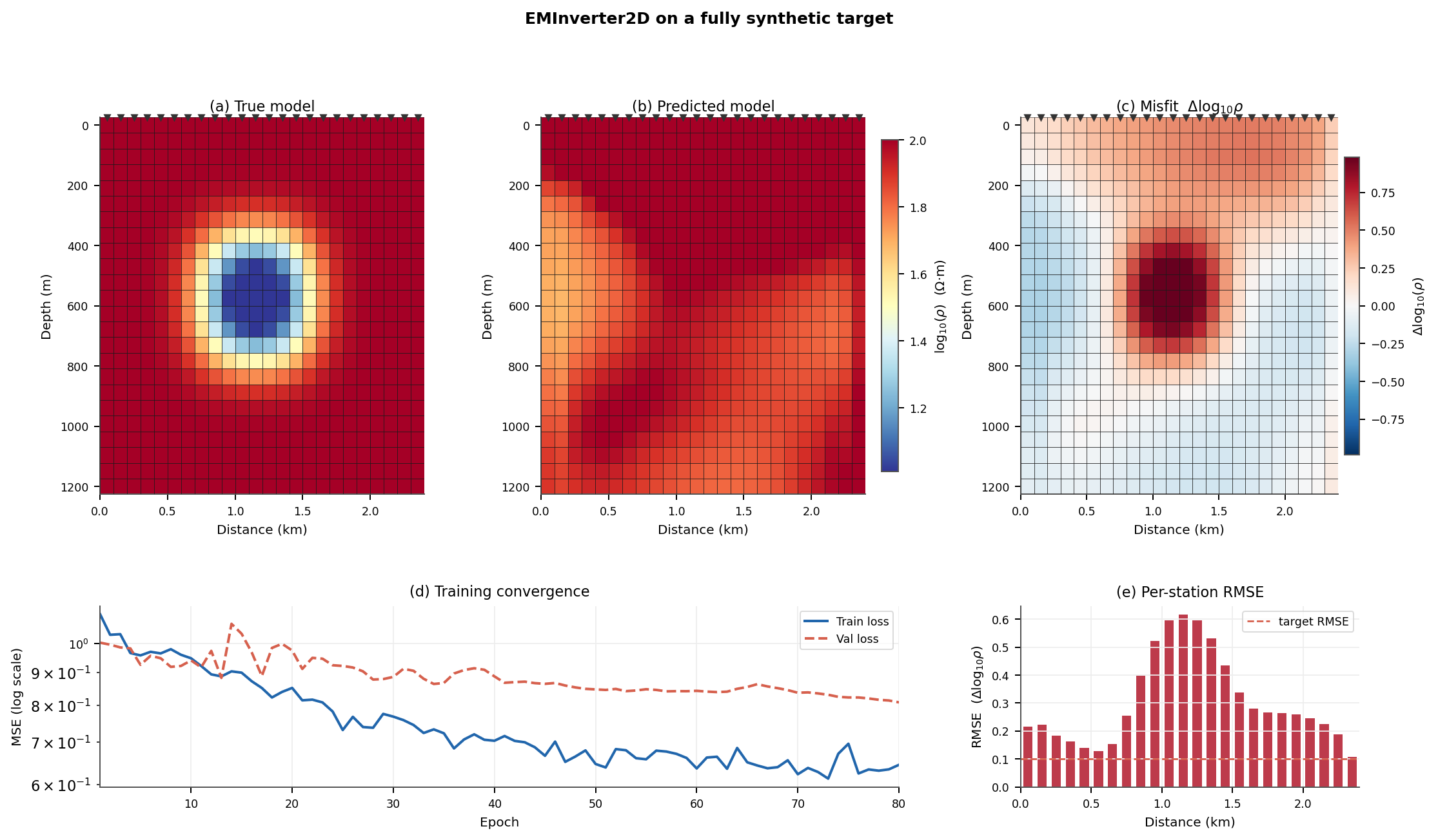
Every panel here shows the section’s mesh (pycsamt.api.mesh.draw_mesh(), preset="review") drawn on top of its color fill – the same overlay available to any section in this guide via show_mesh=True, not something specific to this synthetic example. The true model (a) is a single Gaussian-smoothed conductor, matched in scale to the training correlation lengths so it is not an unfairly out-of-distribution shape. At only a hundred training realizations, the predicted model (b) does not visually isolate that conductor at all – it instead shows a west-heavy resistive gradient the true model does not have. The misfit panel (c) is where the training budget’s real signal shows up: it peaks precisely at the true conductor’s location and shape, which is only possible because the prediction stays close to background exactly there while drifting elsewhere. That is a rejection signal, not a recovery – a hundred realizations captures the pipeline end to end but is not sufficient supervision for the U-Net to separate one compact target from its own gradient artifacts. Rerun the source above with several times the realizations and epochs before treating a predicted section like this one as evidence of anything.

Only the TE zxy response is requested by this agent because its two input channels are \(\log_{10}\rho_a^{xy}\) and \(\phi^{xy}\). The lower-level 2-D dataset machinery can validate TM zyx responses as well, but computing an unused TM solve here would not add a feature to the U-Net. For angular frequency \(\omega=2\pi f\), the complex TE impedance is converted using

(2)\[\rho_a^{xy}(f,x) = \frac{|Z_{xy}(f,x)|^2}{\mu_0\omega}, \qquad \phi^{xy}(f,x) = \operatorname{atan2} \bigl(\Im Z_{xy},\Re Z_{xy}\bigr),\]

which is also the conversion applied by the implementation to the canonical SI impedance returned by the Maxwell adapter. These arrays are transposed into (channel, frequency, station) order, while the target is \(m=\log_{10}\rho\) in (depth, station) order.

On PyTorch, optional spatial penalties augment the normalized target-space mean-squared error. With batch index \(b\), depth cell \(k\), station \(j\), prediction \(\hat m\), and target \(m\), the implemented objective is

(3)\[\begin{split}\begin{aligned} \mathcal L ={}& \frac{1}{N}\sum_{b,k,j} (\hat m_{bkj}-m_{bkj})^2 \\ &+\lambda_x\,\operatorname{mean} (\hat m_{b,k,j+1}-\hat m_{b,k,j})^2 \\ &+\lambda_z\,\operatorname{mean} (\hat m_{b,k+1,j}-\hat m_{b,k,j})^2 \\ &+\lambda_{\mathrm{TV}}\left[ \operatorname{mean}|\hat m_{b,k,j+1}-\hat m_{b,k,j}| +\operatorname{mean}|\hat m_{b,k+1,j}-\hat m_{b,k,j}| \right]. \end{aligned}\end{split}\]

All three weights default to zero, in which case (3) reduces exactly to target-space MSE. The quadratic terms suppress sharp gradients increasingly strongly, whereas total variation permits sharper boundaries but can produce blocky sections. These are learned-model regularizers; they do not turn the inference pass into a classical response-space inversion. TensorFlow currently accepts the plain MSE path only and rejects non-zero spatial weights rather than silently ignoring them.

Ten neighbouring stations share one U-Net input panel, so the predicted section is smooth along the profile by construction — that smoothness comes from the network architecture and training design, not from resolving lateral continuity the way a regularised classical 2-D inversion would. The call above runs on the real, sparse WILLY line and a modest smoke-test budget; run it yourself with a larger n_train_profiles/epochs budget to see the section it converges to on your machine, rather than trusting a single fixed doc-build capture as a stand-in for a validated result.

Important outputs are pred_section with shape (n_depth, n_stations), depths_km, station_names, rms_global, physics, mt2d_recovery, the fitted inverter, and figure dictionaries. mt2d_recovery is None on the tiled path. On the Maxwell path it averages RMSE, MAE, and \(R^2\) over the held-out test split, or the validation split when no test sample exists. Those scores compare predicted and known synthetic \(\log_{10}\rho\); they are a domain-specific recovery audit, not field ground truth.

The reported field RMS is a data-space check: the predicted section is mapped back to an apparent resistivity curve at each station using the Bostick depth \(d_B = 503\sqrt{\rho_a T}\) (the same skin depth relation used elsewhere in pyCSAMT), and compared against the observed log10 apparent resistivity at that station.

With topography=True, the agent extracts elevations and cumulative chainage from the same Sites object, aligns them by the names of the stations retained in the U-Net panel, and adds topography_section to the figure dictionary. Explicit terrain remains available when a collection does not contain elevations:

>>> terrain_result = agent.execute({
...     "sites": sites,
...     "topography": {
...         "elevation_m": measured_elevation,
...         "chainage_km": measured_chainage,
...         "exaggeration": 1.0,
...     },
... })
>>> terrain_result["topography"]["applied"]
True
>>> terrain_result["topography"]["affects_forward_physics"]
False

The compact WILLY example below uses 12 stations, 16 frequency bins, eight depth cells, and measured site topography. Its horizontal coordinate is the approximately 1.10 km measured chainage of the retained stations, rather than the legacy assumed 0.5 km spacing. But it also deliberately trains for only two epochs to keep the documentation build fast — terrain changes the displayed vertical datum, it does not repair that budget or make the U-Net a terrain-aware EM solver. Run the source below yourself with a real epoch count to see a converged terrain-draped section rather than a two-epoch snapshot:

</>View the WILLY Inv2DAgent topography sourceClick to inspect and copy the complete code

def make_agents_inv2d_willy_topography() -> None:
    """Execute a compact WILLY Inv2DAgent terrain-output contract."""
    try:
        import torch

        torch.manual_seed(43)
    except ImportError:
        pass
    np.random.seed(43)
    sites = ensure_sites(
        PROJECT_ROOT / "data" / "AMT" / "WILLY_data" / "L18PLT",
        recursive=True,
        verbose=0,
    )
    dense_features, measured_frequency, _ = sites_to_features_1d(
        sites,
        comp="xy",
        n_freqs=64,
    )
    rho_reference = float(
        10.0 ** np.nanmedian(dense_features[:, : measured_frequency.size])
    )
    frequency_min = max(
        float(measured_frequency.min()),
        float(frequency_for_depth(2000.0, rho_reference)),
    )
    _, frequency, _ = sites_to_features_1d(
        sites,
        comp="xy",
        n_freqs=16,
        freq_min=frequency_min,
        freq_max=float(measured_frequency.max()),
    )
    result = Inv2DAgent(
        n_depth=8,
        freqs=frequency,
        depth_max=2000.0,
        n_train_profiles=8,
        n_stations_per_profile=12,
        epochs=2,
    ).execute({"sites": sites, "topography": True})
    if result.status == "failed":
        raise RuntimeError(result.error)
    fig = result["figures"]["topography_section"]
    fig.set_constrained_layout(False)
    fig.set_size_inches(12.5, 6.2)
    fig.subplots_adjust(left=0.09, right=0.88, bottom=0.14, top=0.70)
    _save(fig, "agents_inv2d_willy_topography.png")

The absolute-elevation transformation is given later by equation (10) and is identical for the 2-D and graph outputs. If elevation is missing, non-finite, flat zero, or cannot be matched after station filtering, the agent keeps the ordinary section and returns a warning instead of presenting artificial flat terrain as measured topography.

Under physics="mt1d", learned lateral continuity comes from the assembled profile and network architecture rather than a 2-D forward operator. Under physics="mt2d", the synthetic responses do contain lateral EM coupling, but the trained U-Net remains an amortized predictor whose field result can be out of distribution. Neither mode proves that the field structure is two-dimensional. Validate the section against dimensionality evidence, held-out recovery, reconstructed field responses, and classical 2-D inversion where feasible.

6.3.20.9. Inv3DAgent: spatial graph workflow

pycsamt.agents.Inv3DAgent represents stations as graph nodes. Edges connect stations within radius unless a normalized adjacency matrix is supplied. When coords is omitted, the agent reads each station’s EDI header coordinates and projects them to local metres:

>>> import numpy as np
>>> from pycsamt.agents import Inv3DAgent
>>> from pycsamt.ai.inversion import sites_to_features_1d
>>> _, measured_frequency, _ = sites_to_features_1d(
...     sites, comp="xy", n_freqs=64,
... )
>>> agent = Inv3DAgent(
...     physics="mt1d",
...     n_layers=10,
...     freqs=np.geomspace(
...         float(measured_frequency.min()),
...         float(measured_frequency.max()),
...         32,
...     ),
...     n_train_profiles=300,
...     epochs=80,
...     radius=250.0,
...     hidden=(256, 128, 64),
...     dropout=0.1,
...     n_mc=50,
... )
>>> result = agent.execute({
...     "sites": sites,
...     "output_dir": "outputs/ai_inversion/survey_3d",
... })
>>> print(result.status, result.summary)
success 3-D GCN inversion (physics=mt1d): 28 stations × 10 layers. RMS 3.875, MC σ computed. 3 figures.

The RMS value above is real, captured output, not an illustrative placeholder – but it is not exactly reproducible from this call alone. Fixing numpy’s and PyTorch’s global seeds before construction, as shown, still leaves this specific pipeline’s synthetic-profile generation and training sensitive to prior random-state consumption elsewhere in the process; treat the number as evidence that training converged to a reasonable fit, not as a value to match digit for digit. This is a real, still-open reproducibility gap in the physics="mt1d" path specifically – unlike generate_2d_maxwell_dataset() and generate_3d_maxwell_dataset(), which derive every stochastic draw from an explicit SeedPlan precisely to avoid it (Reproducible experiment configuration).

Passing freqs explicitly, built from the loaded stations’ own measured band, matters here for the same reason it matters below for physics="mt3d": the class default spans \(10^{-4}\)–\(10^3\) Hz, four orders of magnitude below anything a WILLY-class AMT receiver records, and the Bostick display depth that a five-layer model derives from that default reaches hundreds of kilometres – see Why the frequency grid has to come from the survey below for the arithmetic. This first call still keeps physics="mt1d" to make that path’s other limitation visible: the GCN sees graph context, but its synthetic responses are independent layered-earth columns. It is not the new 3-D Maxwell workflow.

Pass projected coordinates in metres explicitly whenever a project’s own survey geometry or CRS is authoritative; only fall back to the auto-derived layout for exploratory work. The projection is a simple equirectangular approximation in absolute metres, not centred on a local origin, so expect large-magnitude coordinate values — what the radius gate and the figures below care about is the relative spacing between stations, not the absolute numbers.

Real station spacing lets adjacent stations exchange information through the graph, so the resulting section varies smoothly along the line instead of the single flat column produced when every station lands at the same point. With the frequency grid tied to the measured band (as constructed above), the display extends to a defensible ~8 km rather than several hundred, and a laterally discontinuous conductor can stay visible instead of being buried inside an unconstrained mantle-scale axis. This physics="mt1d" route remains a tiled baseline, though — run the call above yourself rather than trusting a fixed capture as the reference result; the genuine 3-D Maxwell route below is the one worth comparing it against.

What physics="mt3d" now executes

The current MT3D route changes the forward physics, not merely the plot label. For each realization, GeologyGrid spans the real station footprint and carries a correlated three-dimensional resistivity field \(\rho_r(x,y,z)\). The dataset builder embeds that core into a padded, non-uniform MaxwellMesh and solves the frequency-domain curl–curl system

(4)\[\nabla\times\nabla\times\mathbf E_r(\omega) + i\omega\mu_0\sigma_r\mathbf E_r(\omega)=0, \qquad \sigma_r=\rho_r^{-1}.\]

MT3DAdapter evaluates equation (4) for two horizontal source polarizations. The training feature at station \(s\) retains the TE-like zxy response on the declared frequency grid,

(5)\[\mathbf x_{r,s} =\left[\log_{10}\boldsymbol\rho_{a,xy}, \boldsymbol\phi_{xy},\mathbf 0\right], \qquad \mathbf y_{r,s} =\left[\log_{10}\rho_r(x_s,y_s,z_1),\ldots, \log_{10}\rho_r(x_s,y_s,z_L)\right].\]

Here the zero block pads the two populated zxy channels to the GCN’s four-channel slot. The resistivity part of the label in equation (5) is sampled from the same 3-D volume that generated the response, while its interface-thickness part is the fixed declared display grid. It is not a tiled 1-D resistivity target. The realization ID remains intact through the train/validation/test split, so different samples from one earth model cannot leak across partitions. Failed Maxwell solves are rejected rather than silently entering training.

The built-in generator samples correlated Gaussian fields controlled by horizontal and vertical correlation-length ranges, log-resistivity mean and spread, and grid resolution. It does not yet draw explicit stratigraphic interfaces, ellipsoidal lenses, faults, or petrophysical classes. Those richer pycsamt.ai.geology objects can define an external training corpus, but raising n_train_profiles alone only adds realizations of the configured Gaussian-field family. Geological diversity and realization count are separate parts of the prior.

The two 3-D forward backends have different roles. The in-process MT3DAdapter now supports padded non-uniform meshes and passes the small-grid half-space and layered-earth benchmarks, but its direct sparse solve remains research-scale. The compiled ModEm3DAdapter is the validated production forward backend and supports larger non-uniform models. The current Maxwell3DDatasetConfig is wired to the in-process adapter, however; setting physics="mt3d" does not silently invoke ModEM. A production ModEM training corpus must be generated explicitly through the solver-neutral Maxwell problem/result contract and then supplied to GCNInverter3D.

Both adapters currently expose a surface-at-mesh-top contract in this API. Although ModEM itself can represent air and topography, the present ModEm3DAdapter deliberately does not map them. Consequently a topographic display from Inv3DAgent is still a coordinate transformation, not evidence that terrain entered equation (4). See Solvers And Grids, Maxwell Forward Modelling and Solver Contracts, and ModEM before moving from the executable research example to a production 3-D study.

Why the frequency grid has to come from the survey

Neither figure above was trained on the class’s own default frequency grid, np.logspace(-4, 3, 32), and that omission is deliberate enough to be worth working through arithmetically. Its minimum frequency is \(10^{-4}\) Hz, or a 10,000-s period, even though WILLY L18 spans only about 1.008–10,400 Hz. The legacy thickness helper takes a 100 \(\Omega\mathrm{m}\) reference and computes

(6)\[d_{\max} = \sqrt{\frac{\rho_{\mathrm{ref}}T_{\max}} {4\pi^2\mu_0}}.\]

For that default grid, equation (6) gives a 355.88 km final thickness. The four finite-layer thicknesses are 3.56, 16.52, 76.67, and 355.88 km, giving cumulative interfaces at 3.56, 20.08, 96.75, and 452.63 km — a mantle-scale axis produced by a training target that was never built from this survey’s actual sensitivity. Every figure on this page that still shows that scale should be read as a parameterization warning, not as WILLY deep geology.

Cropping such an image at 2 km would be misleading, because the GCN would still have been trained against hundreds-of-kilometres thickness targets. The correction has to enter before synthetic generation, which is exactly what both worked examples above do. Inv3DAgent therefore accepts explicit freqs and depth_max values; with \(L-1\) finite layers, the revised thicknesses use positive geometric weights \(w_k\) normalized to the declared model depth,

(7)\[h_k = d_{\max}\frac{w_k}{\sum_{j=1}^{L-1}w_j}, \qquad \sum_{k=1}^{L-1}h_k=d_{\max}.\]

For the five-layer WILLY example, depth_max=2000 m produces interfaces at 0.266, 0.649, 1.202, and 2.000 km. The frequency grid should also come from the loaded survey rather than from hard-coded WILLY endpoints. The public pycsamt.ai.inversion.sites_to_features_1d() bridge returns a common logarithmic grid constructed from the station observations. A depth-oriented frequency associated with the target depth can then be estimated with pycsamt.emtools.frequency_for_depth():

(8)\[\rho_{\mathrm{ref}} =10^{\operatorname{median}(\log_{10}\rho_a)}, \qquad f_D=\rho_{\mathrm{ref}} \left(\frac{356}{D}\right)^2, \qquad f_{\min}=f_{\min}^{\mathrm{obs}}, \qquad f_{\max}=\min(f_{\max}^{\mathrm{obs}},f_D).\]

This is a survey-design heuristic. The apparent-resistivity reference is explicit, and changing it changes \(f_D\). Lower frequencies carry the deeper sensitivity, so the smoke-scale MT3D example retains the lowest measured frequencies and uses \(f_D\) as its upper bound. This choice does not prove a depth of investigation or replace sensitivity kernels. Preserve the full-band data and compare targeted, full-band, and alternative-mesh scenarios before interpretation.

For WILLY L18, a 64-point survey-derived grid spans 1.008–10,400 Hz and has median XY apparent resistivity \(\rho_{\mathrm{ref}}=453.75\) \(\Omega\mathrm{m}\). Equation (8) gives \(f_D=14.38\) Hz for \(D=2000\) m. The executed demonstration therefore intersects the observed support with 1.008–14.38 Hz and constructs three logarithmic points inside that interval. This deliberately small grid keeps the genuine 3-D Maxwell example reproducible on a CPU. The grid and thickness targets are shared by synthetic generation, observed-feature extraction, forward RMS, returned metadata, and plotting:

>>> import numpy as np
>>> from pycsamt.agents import Inv3DAgent
>>> from pycsamt.ai.inversion import sites_to_features_1d
>>> from pycsamt.emtools import frequency_for_depth
>>>
>>> dense_X, measured_frequency, _ = sites_to_features_1d(
...     sites, comp="xy", n_freqs=64,
... )
>>> rho_reference = float(
...     10.0 ** np.nanmedian(dense_X[:, :measured_frequency.size])
... )
>>> frequency_at_2km = float(frequency_for_depth(2000.0, rho_reference))
>>> frequency_min = float(measured_frequency.min())
>>> frequency_max = min(float(measured_frequency.max()), frequency_at_2km)
>>> _, willy_frequency, _ = sites_to_features_1d(
...     sites, comp="xy", n_freqs=3,
...     freq_min=frequency_min,
...     freq_max=frequency_max,
... )
>>> round(rho_reference, 2), round(frequency_at_2km, 2)
(453.75, 14.38)
>>> configured = Inv3DAgent(
...     n_layers=5,
...     freqs=willy_frequency,
...     depth_max=2000.0,
...     n_train_profiles=20,
...     epochs=40,
...     radius=250.0,
...     hidden=(64, 32),
...     n_mc=0,
...     physics="mt3d",
...     geology_grid_nx_ny=4,
...     geology_grid_nz=4,
...     max_mesh_cells=60_000,
... ).execute({
...     "sites": sites,
...     "topography": {
...         "enabled": True,
...         "exaggeration": 1.0,
...         "interp_method": "linear",
...     },
... })
>>> configured.status
'success'
>>> configured.summary
'3-D GCN inversion (physics=mt3d): 28 stations × 5 layers. RMS 4.299. 3 figures. Held-out recovery RMSE=0.495 (log10 Ω·m, n=2).'
>>> configured["frequency_grid_hz"][[0, -1]]
array([ 1.008, 14.37653093])
>>> configured["depths_km"].round(3)
array([0.   , 0.266, 0.649, 1.202, 2.   ])
>>> configured["topography"]["source"]
'sites'
>>> configured["topography"]["affects_forward_physics"]
False
>>> configured["mt3d_recovery"] is not None
True

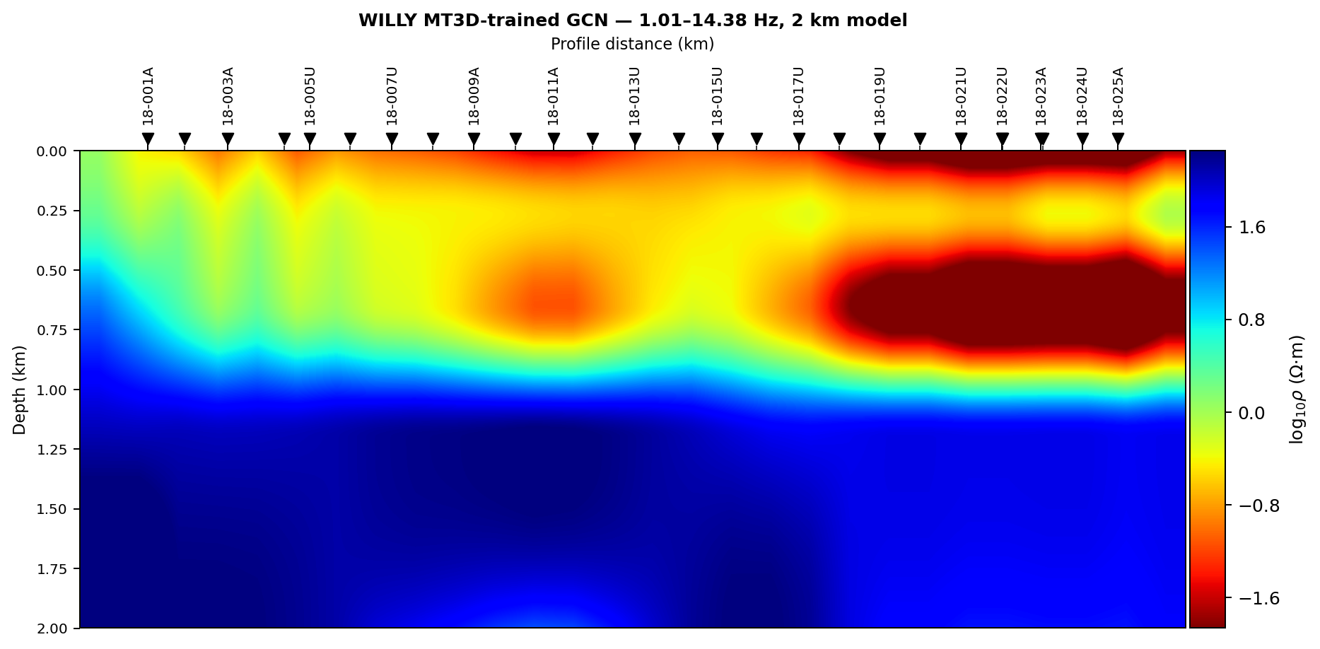
Executed WILLY GCN section trained by Genuine 3-D Maxwell training and evaluated on the real station geometry. The 1.008–14.38 Hz grid samples the deep end of the measured band and the cumulative 2 km bottom is an explicit model boundary, not a claimed depth of investigation. A conductor concentrates beneath the eastern half of the line (stations 18-019U to 18-024U, roughly 0.3–0.8 km depth) under a more resistive near-surface layer – a laterally varying result the tiled physics="mt1d" path structurally cannot produce, since the review below still applies before treating it as a confirmed body.

This corrected scale makes the output appropriate for review, not automatic acceptance. The run uses twenty correlated geological volumes, three frequencies, a \(4\times4\times4\) geology grid, and 40 epochs – enough realizations for the held-out split to carry two independent test volumes instead of one. Every training example is passed through MT3DAdapter; the agent then samples the true volume beneath each real station to form the supervised target. The returned mt3d_recovery report measures held-out error against known synthetic truth. For held-out log-resistivities \(y_i\), predictions \(\hat y_i\), and their target mean \(\bar y\), the report uses

(9)\[\mathrm{RMSE}=\sqrt{\frac{1}{N}\sum_{i=1}^{N}(\hat y_i-y_i)^2}, \qquad \mathrm{MAE}=\frac{1}{N}\sum_{i=1}^{N}|\hat y_i-y_i|, \qquad R^2=1-\frac{\sum_i(\hat y_i-y_i)^2} {\sum_i(y_i-\bar y)^2}.\]

Equation (9) gives RMSE 0.495, MAE 0.396, and \(R^2=-0.544\) over the two held-out volumes. The negative coefficient of determination is a rejection signal, not evidence of useful recovery, and two test volumes are too few to trust the number beyond that binary read. The field-response rms_global moved from 0.981 with four training realizations to 4.299 with twenty – a worse fit to the real WILLY responses despite five times the synthetic training budget. That is not a contradiction to resolve away: Inv3DAgent’s physics="mt3d" path shares the same open reproducibility gap already flagged for physics="mt1d" above, because dataset realizations are drawn from an explicit SeedPlan but network initialization and dropout still consume PyTorch’s global random state, which differs with the surrounding import and execution context. Rerunning this exact call can land on a better or worse field fit than either number here. These settings prove the end-to-end configuration and expose failure modes cheaply; they do not certify the field model, and a production run needs enough realizations and repeated seeds for the recovery and field metrics to stop moving this much between runs.

</>View the WILLY MT3D inversion and topography sourceClick to inspect and copy the complete code

def make_agents_inv3d_willy_2km() -> None:
    """Execute genuine 3-D Maxwell training on the real WILLY geometry."""
    try:
        import torch

        torch.manual_seed(73)
    except ImportError:
        pass
    np.random.seed(73)
    sites = ensure_sites(
        PROJECT_ROOT / "data" / "AMT" / "WILLY_data" / "L18PLT",
        recursive=True,
        verbose=0,
    )
    dense_features, measured_frequency, _ = sites_to_features_1d(
        sites,
        comp="xy",
        n_freqs=64,
    )
    rho_reference = float(
        10.0 ** np.nanmedian(dense_features[:, : measured_frequency.size])
    )
    depth_frequency = float(frequency_for_depth(2000.0, rho_reference))
    frequency_min = float(measured_frequency.min())
    frequency_max = min(float(measured_frequency.max()), depth_frequency)
    _, frequency, _ = sites_to_features_1d(
        sites,
        comp="xy",
        n_freqs=3,
        freq_min=frequency_min,
        freq_max=frequency_max,
    )
    result = Inv3DAgent(
        n_layers=5,
        freqs=frequency,
        depth_max=2000.0,
        n_train_profiles=20,
        epochs=40,
        radius=250.0,
        hidden=(64, 32),
        dropout=0.1,
        n_mc=0,
        physics="mt3d",
        geology_grid_nx_ny=4,
        geology_grid_nz=4,
        max_mesh_cells=60_000,
    ).execute({"sites": sites, "topography": True})
    if result.status == "failed":
        raise RuntimeError(result.error)
    print(
        "agents_inv3d_willy_2km.png",
        ascii(result.summary),
        "recovery=",
        ascii(result.get("mt3d_recovery")),
    )
    fig = result["figures"]["resistivity_section"]
    ax = fig.axes[0]
    ax.set_title(
        f"WILLY MT3D-trained GCN — {frequency[0]:.2f}–"
        f"{frequency[-1]:.2f} Hz, 2 km model",
        fontsize=10,
        fontweight="bold",
    )
    ax.xaxis.set_label_position("top")
    ax.xaxis.tick_top()
    _save(fig, "agents_inv3d_willy_2km_section.png")

Interpret conductors only where response reconstruction, dimensionality, regularization sensitivity, and independent geology agree. Also avoid calling 2 km the depth of investigation merely because it is now the configured model bottom.

The same execution can now obtain elevation and chainage from the supplied Sites object. It aligns terrain by station name after unusable stations have been removed, rather than truncating the elevation array by position. The returned station_elevation_m values are metres above sea level and station_chainage_km is cumulative profile distance. These arrays place each station marker on the terrain surface and transform depth below ground into absolute elevation,

(10)\[z_{j,k}^{\mathrm{abs}} = \frac{E_j}{1000} - d_k,\]

where \(E_j\) is station elevation in metres above sea level and \(d_k\) is positive-down model depth in kilometres. Equation (10) is a coordinate transformation, not a topographic correction to the MT equations. The training responses now come from the 3-D Maxwell solver, but terrain is still applied only when the predicted section is rendered, which is why the result records affects_forward_physics=False. A terrain-aware inversion would require air cells or a topographic finite-element/finite-difference mesh in both training and response reconstruction.

The same run also produces a terrain-draped topography_section figure (built by the code-dropdown above). The 37–144 m WILLY relief is modest compared with the 2 km model, yet its inclusion makes the vertical datum unambiguous: stations follow the profile surface across 2.42 km of chainage, and resistivity cells extend downward from that local surface. Vertical exaggeration should remain at one for depth comparison, and any larger value must be described as a display choice, not a fresh solve.

Outputs include pred_rho in log10 resistivity, pred_thick in log10 metres, optional pred_uncertainty, depths_km, coordinates, adjacency, edge count, global RMS, figures, and the inverter. Internally, the adjacency matrix follows the same renormalisation used by Kipf & Welling (2017) for spectral graph convolutions: with \(A\) the raw within-radius connectivity, self-loops are added and the result is symmetrically normalised,

(11)\[\tilde{A} = A + I, \qquad \hat{A} = \tilde{D}^{-1/2}\,\tilde{A}\,\tilde{D}^{-1/2},\]

where \(\tilde D\) is the diagonal degree matrix of \(\tilde A\). A larger radius densifies \(\hat A\) and lets the network average over more distant, possibly unrelated, structure.

The reported rms_global needs a precise boundary. Even when training uses physics="mt3d", the current field-response audit converts each predicted station column to a LayeredModel and evaluates it with MT1DForward. It is therefore the mean of station-wise 1-D apparent-resistivity residuals, not a coupled 3-D reconstruction through MT3DAdapter or ModEM. Use it as a quick inconsistency screen. A production release still requires a full 3-D forward reconstruction of the assembled volume on the same stations, components, frequencies, error floors, and mesh policy used by the declared validation protocol.

output_dir writes generated figures but does not currently serialize the fitted GCN automatically. Save it explicitly while the returned inverter is still available, then verify a fresh-process reload before treating it as a checkpoint:

>>> from pathlib import Path
>>> from pycsamt.ai.inversion import GCNInverter3D
>>> checkpoint = Path("outputs/ai_inversion/survey_3d/gcn_mt3d.npz")
>>> configured["inverter"].save(checkpoint)
>>> restored = GCNInverter3D.load(checkpoint)
>>> checkpoint.exists()
True

The checkpoint preserves network parameters and fitted weights. Preserve the frequency grid, station order, coordinate reference, adjacency radius or matrix, depth parameterization, geology/dataset manifest, solver identity, mesh policy, split IDs, and normalization metadata beside it; the weight file alone cannot reconstruct the scientific experiment.

pred_uncertainty is Monte Carlo dropout standard deviation across \(M\) stochastic passes with dropout kept active at inference time,

(12)\[\sigma_\ell = \sqrt{\frac{1}{M}\sum_{m=1}^{M} \bigl(\hat y_\ell^{(m)} - \bar y_\ell\bigr)^2}, \qquad \bar y_\ell = \frac{1}{M}\sum_{m=1}^{M} \hat y_\ell^{(m)},\]

for layer index \(\ell\). It represents one model-based uncertainty component — an epistemic uncertainty estimate — and it does not include training-prior misspecification, coordinate error, inversion non-uniqueness, or field domain shift.

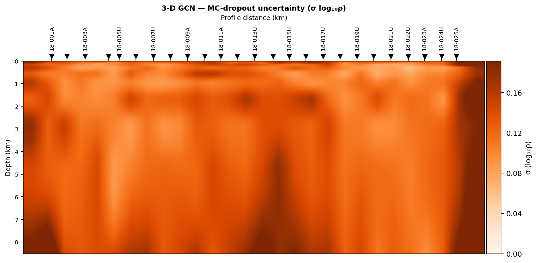
WILLY L18 is essentially a single line of stations, so a plan-view \(E\)–\(N\) uncertainty map would triangulate over near-collinear points and degenerate to a sliver with nothing to fill outside it. The agent detects that profile-like geometry and renders the same distance-vs-depth projection as the resistivity section instead, which is where the spread actually has room to vary.

Check graph connectivity explicitly:

>>> adjacency = result["adjacency"]
>>> degree = (adjacency > 0).sum(axis=1) - 1
>>> print("Graph degree by station:", degree)
Graph degree by station: [1 2 2 3 2 3 2 2 2 2 2 2 2 2 2 2 2 2 2 3 4 4 5 5 4 4 3 1]

The two line endpoints have the lowest degree (1), most interior stations sit at degree 2, and a cluster near stations 20–25 climbs to degree 4–5 — evidence that the real survey line is not evenly spaced and bends or bunches stations more closely together there. Compare this against the field station layout before trusting the graph: disconnected or weakly connected stations cannot receive the intended spatial context, and a very large radius can oversmooth across unrelated structures.

6.3.20.10. EnsembleAgent: uncertainty-aware 1-D workflow

pycsamt.agents.EnsembleAgent trains independent 1-D estimators with different seeds and returns prediction intervals:

>>> from pycsamt.agents import EnsembleAgent
>>> agent = EnsembleAgent(
...     n_estimators=5,
...     arch="resnet",
...     n_layers=5,
...     n_train_samples=2_000,
...     epochs=30,
...     calibrate=True,
... )
>>> result = agent.execute({
...     "sites": sites,
...     "output_dir": "outputs/ai_inversion/L18_ensemble",
... })
>>> print(result.status, result.summary)
success Ensemble inversion (5× resnet): 28 stations. RMS=2.149. 90% coverage=6.2%. 2 figures.

Inspect pred_mean, pred_std, pred_lo, pred_hi, coverage, and rms_global. Calibration follows split conformal prediction (Vovk et al. 2005): each ensemble member gives a mean \(f(\mathbf{x})_j\) and a per-parameter spread \(\sigma_j(\mathbf{x})\), and a held-out calibration set fixes one quantile of the normalised residuals,

(13)\[s_i = \max_j \frac{\lvert y_{ij} - f(\mathbf{x}_i)_j\rvert}{\sigma_j(\mathbf{x}_i) + \varepsilon}, \qquad \hat q = \operatorname{Quantile}_{1-\alpha+\frac{1}{n_{\mathrm{cal}}+1}}(s_1,\dots,s_{n_{\mathrm{cal}}}),\]

so that a new interval

(14)\[\bigl[f(\mathbf{x})_j - \hat q\,\sigma_j(\mathbf{x}),\; f(\mathbf{x})_j + \hat q\,\sigma_j(\mathbf{x})\bigr]\]

carries a marginal coverage guarantee of \(1-\alpha\) — but only under exchangeability between the calibration set and the inputs it is applied to.

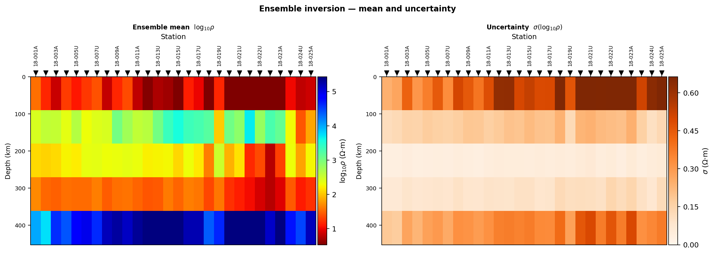
The current uncertainty panel reaches approximately \(\sigma=0.67\) in shallow cells. That visible spread is still poorly calibrated: the nominal 90% interval covers only 6.2% of the held-out synthetic targets.

That last point is not a footnote. This five-member, 30-epoch-per-member ensemble remains far below its nominal coverage, and its predicted cumulative depth again extends beyond 400 km. Bounds represent the agent’s ensemble and optional calibration procedure, conditional on its synthetic distribution — empirical coverage on held-out synthetic examples is not automatically field coverage, and this run is a direct demonstration of that gap rather than a hypothetical one. More estimators, more training per estimator, and a larger calibration set are the usual first response before trusting a reported coverage number.

6.3.20.11. PINNInversionAgent

pycsamt.agents.PINNInversionAgent supports dimensions 1, 2, and 3 and optimizes a physics-informed inversion loss without labelled model targets:

>>> from pycsamt.agents import PINNInversionAgent
>>> agent = PINNInversionAgent(
...     dim=2,
...     n_layers=10,
...     depth_max=2000.0,
...     smoothness_weight=0.01,
...     lateral_weight=0.005,
...     epochs=300,
...     lr=1e-2,
...     solver="mt1d",
... )
>>> result = agent.execute({
...     "sites": sites,
...     "output_dir": "outputs/ai_inversion/L18_pinn2d",
... })
PINNInverter2D: optimising 28 stations x 10 layers (300 epochs) ...
  epoch    50/300  loss=1.22558
  epoch   100/300  loss=1.05607
  epoch   150/300  loss=0.93819
  epoch   200/300  loss=0.83882
  epoch   250/300  loss=0.77421
  epoch   300/300  loss=0.74359
>>> print(result.status, result.summary)
success PINN-2D: 28 stations, 10 layers. RMS 0.693. 2 figure(s).

Outputs include section, optional layered models for 1-D, rms_per_station, rms_global, loss and residual dataframes when available, figures, and the fitted inverter. No synthetic labelled dataset was generated for this run; every cell is fit directly against the physics-informed residual for that station, which is why the loss trace above — not a labelled-recovery score — is the primary evidence of fit quality here. Run the call above yourself to inspect the resulting section directly rather than relying on a single archived capture of it.

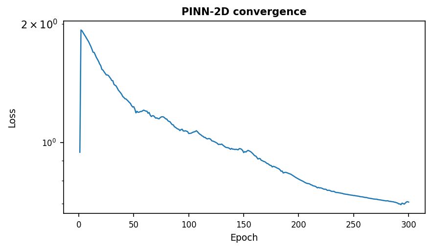
The loss trace above is the same descent printed to the console; reviewing both the numbers and the curve catches a run that stopped improving long before its epoch budget ran out.

This 300-epoch figure is an archived successful run, whereas the shorter executed smoke test in Physics-informed 2-D inversion increased its objective and was rejected. The two outcomes are not interchangeable evidence. They demonstrate why the manifest must preserve initialization, backend, learning rate, epoch count, station order, and software revision, and why a stored figure without its numeric loss and residual tables is insufficient for reproduction.

Physics-informed does not mean assumption-free. Solver dimension, regularization weights, depth parameterization, optimizer, learning rate, and stopping behavior all condition the result. See Physics-informed 2-D inversion for the full scientific workflow.

6.3.20.12. ModelZooAgent

List Model zoo registry metadata without downloading weights:

>>> from pycsamt.agents import ModelZooAgent
>>> zoo = ModelZooAgent()
>>> listed = zoo.execute({"action": "list"})
>>> for item in listed["details"]:
...     print(item["name"], item["arch"], item["n_layers"])
mt1d-resnet-5layer-v1 resnet 5
mt1d-cnn-5layer-v1 cnn1d 5
mt1d-resnet-7layer-v1 resnet 7
csamt1d-resnet-5layer-v1 resnet 5
tem1d-fcn-5layer-v1 fcn 5

Download and prediction actions require model_name:

>>> downloaded = zoo.execute({
...     "action": "download",
...     "model_name": "mt1d-resnet-5layer-v1",
... })
>>> print(downloaded.status)
needs_review
>>> print(downloaded.warnings[0])
Failed to download '.../mt1d-resnet-5layer-v1.npz': HTTP Error 404: Not Found
Pre-trained weights for pycsamt are scheduled for Phase 5 and may not yet be
publicly available. Train your own model with EMInverter1D.fit() or check
https://github.com/earthai-tech/pycsamt-models for updates.

Weights for this registry entry are not released yet, so download reports needs_review rather than a silent success. predict falls back to on-the-fly training when that happens:

>>> predicted = zoo.execute({
...     "action": "predict",
...     "model_name": "mt1d-resnet-5layer-v1",
...     "sites": sites,
...     "output_dir": "outputs/ai_inversion/zoo_prediction",
... })
>>> print(predicted.status, predicted.get("checkpoint_path"), round(predicted.get("rms_global"), 3))
success None 1.29

Check exact status and checkpoint_path. Here checkpoint_path is None and the RMS matches a fresh 2,000-sample, 30-epoch fit — confirming in the result itself, not just in a warning, that no pretrained weights were actually used. Confirm warnings and provenance before describing a result as pretrained.

6.3.20.13. Checkpoint and output policy

An approved AI run should preserve:

• input survey and QC identifiers;

• exact agent class and constructor parameters;

• runtime payload and overrides;

• backend, dependency versions, hardware, and seeds;

• synthetic dataset configuration or checkpoint identity and checksum;

• training history and stopping behavior;

• prediction arrays in their documented units;

• station ordering, frequencies, coordinates, and adjacency where applicable;

• RMS definition and per-station diagnostics;

• ensemble or dropout uncertainty settings;

• all warnings and failures;

• figure paths and a serialized machine-readable result summary;

• reviewer, validation evidence, status, and date.

Most of these belong on a dataset card and model card rather than in ad-hoc notes, so the same identifiers reappear across runs. Do not rely only on the live inverter object stored in AgentResult.data. Save the supported checkpoint plus a plain configuration and manifest that can be inspected without unpickling arbitrary objects.

6.3.20.14. Optional LLM interpretation

Passing api_key, model, and llm_provider enables an optional text interpretation. Without an API key, science execution still runs and llm_interpretation remains None — every run captured on this page used no API key, and each one logged an “LLM query failed” line before continuing normally, which is the intended degrade-gracefully behaviour rather than a failure of the science step.

Treat generated text as a draft. Verify every station count, RMS, depth, geological claim, and recommendation against structured outputs. Do not send sensitive project data to an external provider unless authorized by project policy.

6.3.20.15. Failure handling

Use a consistent guard:

>>> result = agent.execute(payload)
>>> if result.status == "failed":
...     print("Failure:", result.error)
...     print("Remediation:", result.error_fix_hint)
... elif result.status == "needs_review":
...     print("Review required:", result.summary)
...     for warning in result.warnings:
...         print(" -", warning)
... else:
...     for warning in result.warnings:
...         print("Warning:", warning)
...     # Continue to scientific validation.

A missing input fails immediately rather than starting an expensive run:

>>> AIInversionAgent().execute({}).status
'failed'
>>> AIInversionAgent().execute({}).error
"No 'sites' or 'path'."

Common failure causes include no installed deep-learning backend, no input path or sites, unusable impedance, insufficient valid stations, incompatible frequency coverage, disconnected graphs, checkpoint incompatibility, resource exhaustion, and figure-save errors.

Agent success means the programmed workflow returned. It does not mean the model passed scientific acceptance criteria — the ensemble run earlier in this page reported "success" with 0% empirical coverage.

6.3.20.16. Choosing the right interface

Use an agent when:

• the built-in synthetic training assumptions match the project;

• standard EDI-to-result orchestration is desired;

• consistent figures and AgentResult outputs are useful;

• a baseline or screening workflow is being established.

Use pycsamt.ai.inversion directly when:

• training priors or noise models must be customized;

• train, validation, calibration, and test splits require precise control;

• network or loss functions are being researched;

• checkpoint and optimizer behavior must be managed explicitly;

• custom metrics, callbacks, or distributed training are required;

• agent fallbacks are inappropriate for controlled production.

Use the workflow orchestrator only when multiple reviewed steps must be chained. Understand each individual result contract before hiding it inside a larger pipeline.

6.3.20.17. Review checklist

Check	Evidence
Correct agent selected	Survey geometry, dimensionality, target, and architecture rationale.
Input data reviewed	QC, components, frequency coverage, coordinates, processing, and usable station count.
Training provenance retained	Priors, noise, solver, sample count, split, seed, epochs, and history.
Checkpoint identity proven	Model name/path, metadata, checksum, compatibility, and no silent fallback.
Result contract inspected	Exact status, warnings, units, shapes, station order, figures, and paths.
Response fit reviewed	Per-station diagnostics, RMS definition, phase/component limitations, and structured residuals.
Spatial assumptions checked	2-D dimensionality or 3-D coordinates, radius, adjacency, and connectivity.
Uncertainty interpreted conditionally	Ensemble/dropout method, calibration evidence, domain shift, and omitted sources.
Independent validation completed	Classical baseline, synthetic holdout, field response, boreholes, and geological consistency.
Release is auditable	Configuration, checkpoint, outputs, manifest, reviewer, status, and limitations.

6.3.20.18. Common mistakes

Avoid these errors:

• treating agent orchestration as a substitute for AI model validation;

• using default synthetic priors without checking field representativeness;

• ignoring a successful result’s warnings;

• assuming best_model means lowest-error station;

• reporting the 1-D log-resistivity RMS as a full impedance RMS;

• calling U-Net lateral continuity proof of 2-D earth structure;

• accepting the auto-derived coordinate layout without checking it against known survey geometry, especially for CRS or projection assumptions the fallback does not know about;

• assuming period_range narrows the frequency grid on Inv2DAgent or Inv3DAgent — these implementations currently read the explicit freqs override instead, so convert a reviewed period band to frequencies before constructing or executing the agent;

• treating MC dropout or ensemble spread as total uncertainty, especially when a calibration check has not been run against it;

• claiming pretrained inference after a fallback training run;

• trusting generated LLM interpretation without checking structured outputs;

• preserving figures but not the configuration, checkpoint, or data contract;

• continuing automatically after needs_review in a controlled workflow.

6.3.20.19. Next steps

Continue with:

• AI inversion data preparation for representative training and field datasets;

• Training AI inversion models for controlled lower-level model fitting;

• AI inversion inference for checkpoint compatibility and field prediction;

• AI inversion validation for acceptance tests and classical baselines;

• AI inversion uncertainty for predictive calibration and domain shift;

• AI inversion reporting for model cards and release packages;

• Agents for the complete pyCSAMT agent architecture.