9.4. Controlled-Source Edge QC (CSAMT / CSEM)#

Natural-source AMT/MT diagnostics (AMT/CSAMT Edge Diagnostics) assume a plane-wave field with no operator-controlled transmitter. Controlled-source methods, especially CSAMT and CSEM, add a grounded dipole transmitter. That changes the field questions at the edge: is the receiver far enough from the source for a plane-wave interpretation, is there resolvable energy at every transmitted line, and is the source current steady enough to trust the sounding? The pycsamt.iot.edge_csamt and pycsamt.iot.edge_csem modules answer these questions with numpy-only checks on short edge windows, reusing the same spectral helpers as pycsamt.iot.edge_amt.

A transmitter device role and a source telemetry packet let a transmitter node report its state alongside the receivers. The examples below use synthetic data so the same outputs can be reproduced without an EDI file or a field logger export.

9.4.1. Synthetic Controlled-Source Window#

This first block creates one CSAMT-like receiver window and matching transmitter telemetry. The expected transmitter frequency comb is 8, 32, 128, and 512 Hz, but the synthetic signal only contains the first three lines — that deliberate missing line is what makes the frequency-comb check below worth running. The CSEM amplitude curve also contains a small bump at 6000 m so the monotonic-decay check has something real to flag.

>>> import numpy as np
>>> rng = np.random.default_rng(51)
>>> sample_rate = 2048.0
>>> n_samples = 8192
>>> t = np.arange(n_samples) / sample_rate
>>> tx_frequencies = np.array([8.0, 32.0, 128.0, 512.0])
>>> window = (
...     0.18 * np.sin(2 * np.pi * 8.0 * t)
...     + 0.32 * np.sin(2 * np.pi * 32.0 * t)
...     + 0.24 * np.sin(2 * np.pi * 128.0 * t)
...     + 0.035 * rng.standard_normal(n_samples)
... )
>>> tx_current = (
...     9.8 + 0.08 * np.sin(2 * np.pi * 0.6 * t)
...     + 0.03 * rng.standard_normal(n_samples)
... )
>>> tx_voltage = 248.0 + 1.2 * rng.standard_normal(n_samples)
>>> offsets_m = np.array([1000, 2000, 4000, 6000, 8000, 10000], dtype=float)
>>> amplitudes = np.array([8.0e-12, 4.1e-12, 2.1e-12, 2.7e-12, 7.0e-13, 2.0e-13])
>>> phases = np.array([-8.0, -16.0, -29.0, -44.0, -61.0, -79.0])

9.4.2. Skin-Depth Field Zones#

The controlling CSAMT quantity is not offset alone, but the transmitter-receiver offset expressed in skin depth units. For resistivity \(\rho\) in \(\Omega\,m\) and frequency \(f\) in Hz, pyCSAMT uses

\[\delta(f) = 503.29\sqrt{\frac{\rho}{f}}, \qquad q(f)=\frac{r}{\delta(f)}.\]

Here \(r\) is the transmitter-receiver separation and \(q\) is the offset ratio. A frequency is labelled near when \(q \le 1\), far when \(q \ge 3\), and transition between those limits. High frequencies have smaller skin depth, so they usually reach the far field first — which is exactly why the sweep below runs from 4096 Hz down to 1 Hz rather than the other way around.

>>> from pycsamt.iot import classify_field_zones
>>> freqs = np.array([4096.0, 1024.0, 256.0, 64.0, 16.0, 4.0, 1.0])
>>> cov = classify_field_zones(freqs, resistivity=100.0, offset_m=5000.0)
>>> for f, d, ratio, zone in zip(cov.freq_hz, cov.skin_depth_m, cov.offset_ratio, cov.zones):
...     print(f"{f:7.1f} Hz  skin={d:8.1f} m  r/delta={ratio:5.2f}  zone={zone}")
 4096.0 Hz  skin=    78.6 m  r/delta=63.58  zone=far
 1024.0 Hz  skin=   157.3 m  r/delta=31.79  zone=far
  256.0 Hz  skin=   314.6 m  r/delta=15.90  zone=far
   64.0 Hz  skin=   629.1 m  r/delta= 7.95  zone=far
   16.0 Hz  skin=  1258.2 m  r/delta= 3.97  zone=far
    4.0 Hz  skin=  2516.5 m  r/delta= 1.99  zone=transition
    1.0 Hz  skin=  5032.9 m  r/delta= 0.99  zone=near
>>> print(f"all_far_field: {cov.all_far_field}")
all_far_field: False
>>> print(f"correction_recommended: {cov.correction_recommended}")
correction_recommended: True
>>> print(f"first_far_field_hz: {cov.first_far_field_hz():.1f}")
first_far_field_hz: 16.0

Five of the seven rows clear the far-field ratio of 3 comfortably, some by more than an order of magnitude. The two low-frequency rows are the ones to treat carefully: 4 Hz lands at r/delta = 1.99, inside the transition band, and 1 Hz at 0.99 is just barely inside the near field. A near-field correction is recommended the moment either row appears, which is why correction_recommended is True here even though most of the sweep is safely far field.

9.4.3. Transmitter Frequency Comb#

CSAMT transmits a discrete frequency comb rather than the continuous natural spectrum used by passive AMT/MT. For each expected line \(f_k\), pyCSAMT compares the peak power spectral density inside a narrow band around \(f_k\) with the median positive PSD floor \(P_{50}\):

\[\operatorname{SNR}_k = 10\log_{10}\left(\frac{\max P(f \approx f_k)}{P_{50}}\right).\]

A line is detected when that SNR reaches the configured threshold and the line is below Nyquist.

>>> from pycsamt.iot import detect_transmitter_frequencies
>>> comb = detect_transmitter_frequencies(
...     window, sample_rate=sample_rate, tx_frequencies=tx_frequencies,
...     snr_threshold_db=8.0,
... )
>>> print(f"detected lines: {comb.n_detected} of {comb.n_expected}")
detected lines: 3 of 4
>>> print(f"missing lines: {comb.missing()}")
missing lines: [512.0]
>>> for line in comb.lines:
...     print(f"{line.frequency_hz:6.1f} Hz  snr={line.snr_db:6.2f} dB  detected={line.detected}")
   8.0 Hz  snr= 25.89 dB  detected=True
  32.0 Hz  snr= 35.50 dB  detected=True
 128.0 Hz  snr= 32.98 dB  detected=True
 512.0 Hz  snr=  0.87 dB  detected=False

The three lines that were actually built into window all clear the 8 dB threshold by more than 25 dB — the comb detector is not marginal about them. The 512 Hz line, never added to the synthetic signal in the first place, reports 0.87 dB: indistinguishable from the noise floor, exactly as a genuinely silent transmitter line should look. This is the one deliberately planted failure on the page, and the detector finds it without being told which line was missing.

9.4.4. Source-Signal Stability#

The transmitter current sets the signal level of every sounding, so its steadiness bounds the receiver-side data quality. The source-stability check first identifies the on-state samples as those above a fraction of the peak absolute current. On those samples it reports the mean current \(\bar I\), the coefficient of variation

\[\mathrm{CV}_I = \frac{\operatorname{std}(I_\mathrm{on})} {|\operatorname{mean}(I_\mathrm{on})|},\]

and a simple drift amplitude, estimated as the absolute slope of on-state current versus sample index multiplied by the number of on-state samples. A source is unstable when the current CV exceeds max_cv or when no finite current is present.

>>> from pycsamt.iot import assess_source_stability
>>> status = assess_source_stability(tx_current, tx_voltage=tx_voltage)
>>> print(f"stable: {status.stable}")
stable: True
>>> print(f"current_mean_a: {status.current_mean_a:.3f}")
current_mean_a: 9.810
>>> print(f"current_cv: {status.current_cv:.4f}")
current_cv: 0.0066
>>> print(f"current_drift_a: {status.current_drift_a:.3f}")
current_drift_a: 0.005
>>> print(f"on_fraction: {status.on_fraction:.2f}")
on_fraction: 1.00
>>> print(f"voltage_mean_v: {status.voltage_mean_v:.2f}")
voltage_mean_v: 247.98

A CV of 0.0066 is well inside the default max_cv = 0.05, and on_fraction = 1.00 says the synthetic transmitter never keyed off during this window, so every sample counts toward the on-state statistics. This particular source is easy to trust; a transmitter with a failing power supply or a loose ground connection would instead show a current CV rising toward, then past, max_cv.

9.4.5. CSEM Offset Response#

CSEM records a dipole source with a receiver array, and its signature edge product is the response as a function of offset at each frequency. field_vs_offset() builds the magnitude-versus-offset and phase-versus-offset curve, finds the detectability limit, and checks that detectable amplitude decays monotonically with offset.

For detectable amplitudes \(A_i\), the dynamic range is

\[D_\mathrm{dB} = 20\log_{10} \left(\frac{\max(A_i)}{\min(A_i)}\right).\]

The monotonic check allows a small tolerance \(\tau\) and flags a reading when \(A_{i+1} > A_i(1+\tau)\). A bump can mean a bad receiver, a geometry error, or real 3-D structure worth revisiting.

>>> from pycsamt.iot import field_vs_offset
>>> resp = field_vs_offset(
...     offsets_m=offsets_m, amplitudes=amplitudes, phases_deg=phases,
...     noise_floor=1e-13, frequency_hz=1.0,
... )
>>> print(f"n_detectable: {resp.n_detectable} of {resp.n_offsets}")
n_detectable: 6 of 6
>>> print(f"max_detectable_offset_m: {resp.max_detectable_offset_m:.0f}")
max_detectable_offset_m: 10000
>>> print(f"monotonic_decay: {resp.monotonic_decay}")
monotonic_decay: False
>>> print(f"dynamic_range_db: {resp.dynamic_range_db:.2f}")
dynamic_range_db: 32.04
>>> print(f"above_noise: {resp.above_noise}")
above_noise: [True, True, True, True, True, True]

Every offset stays above the \(10^{-13}\) noise floor, so n_detectable is a clean 6 of 6 and the reported dynamic range spans the full curve. monotonic_decay is False for exactly the reason the synthetic data was built that way: the amplitude at 4000 m (\(2.1\times10^{-12}\)) rises to \(2.7\times10^{-12}\) at 6000 m, a 29% jump that clears the default 5% monotonic_tol easily, before the curve resumes its decay out to 10000 m. A real bump of that shape at one offset, surrounded by an otherwise clean decay, is a much stronger signal of a local problem — a bad receiver, a geometry error — than a gently increasing trend would be.

9.4.6. Transmitter Telemetry#

A transmitter node reports its state as a source packet, parsed by the SourcePayload schema with the same tolerant alias folding and range validation as the other payloads. In the example below, current, tx_voltage, frequency, ab_m, and tx_rx_offset are all normalised to canonical payload fields.

>>> from pycsamt.iot import DeviceConfig, FieldSession, parse_payload
>>> tx = DeviceConfig("tx-1", role="transmitter")
>>> payload = parse_payload("source", {
...     "tx_id": "TX1", "current": 9.8, "tx_voltage": 250.0,
...     "frequency": 32.0, "ab_m": 100.0, "tx_rx_offset": 5000.0,
... })
>>> session = FieldSession("CS1", method="csamt", devices=[tx])
>>> _ = session.add_packet({
...     "device_id": "tx-1", "timestamp": 10.0, "topic": tx.topic("source"),
...     "kind": "source", "payload": payload.as_dict(),
... })
>>> print(
...     "payload current/frequency/offset: "
...     f"{payload.tx_current_a:.1f} A, {payload.tx_frequency_hz:.1f} Hz, {payload.offset_m:.0f} m"
... )
payload current/frequency/offset: 9.8 A, 32.0 Hz, 5000 m
>>> print(f"session packets: {len(session.packets)}")
session packets: 1

The raw payload keys (current, tx_voltage, frequency, tx_rx_offset) never appear again after parse_payload runs — every downstream read goes through the canonical tx_current_a, tx_voltage_a, tx_frequency_hz, and offset_m attributes, so a transmitter reporting under a slightly different vendor-specific key name would parse into exactly the same shape.

9.4.7. Static Shift Estimate#

A galvanic static shift multiplies apparent resistivity by a frequency-independent factor while leaving phase nearly unchanged. pyCSAMT estimates the per-period log split between the xy and yx modes,

\[s_i = \log_{10}\rho_{xy,i} - \log_{10}\rho_{yx,i}, \qquad G = 10^{\operatorname{median}(s_i)}.\]

The result is a static-shift candidate when the median split is large enough, the standard deviation of \(s_i\) is small enough, and the mean phase difference stays below the phase threshold.

>>> periods = np.logspace(-3, 1, 12)
>>> res_yx = 80.0 * (1 + 0.08 * np.sin(np.linspace(0, np.pi, periods.size)))
>>> res_xy = 3.0 * res_yx
>>> phi_yx = 42.0 + 1.5 * np.sin(np.linspace(0, 2 * np.pi, periods.size))
>>> phi_xy = phi_yx + 1.2
>>> from pycsamt.iot import estimate_static_shift
>>> ss = estimate_static_shift(res_xy, res_yx, phase_xy=phi_xy, phase_yx=phi_yx)
>>> print(f"static_shift: {ss.static_shift}")
static_shift: True
>>> print(f"shift_factor: {ss.shift_factor:.2f}")
shift_factor: 3.00
>>> print(f"split_decades: {ss.split_decades:.3f}")
split_decades: 0.477
>>> print(f"consistency_std: {ss.consistency_std:.3f}")
consistency_std: 0.000
>>> print(f"phase_diff_deg: {ss.phase_diff_deg:.2f}")
phase_diff_deg: 1.20

res_xy was built as exactly three times res_yx at every period, so the recovered shift_factor of 3.00 is not a coincidence — it is the constant this synthetic data was designed to hide, and consistency_std: 0.000 confirms the split is perfectly frequency-independent because both curves share the same oscillation before the multiplication. The 1.2-degree constant offset added to phi_xy stays far under the default 10-degree phase threshold, which is what a true galvanic distortion should look like: parallel resistivity curves on a log scale with matching phase.

9.4.8. Transmitter Timing Lock#

A CSAMT/CSEM receiver can also report its transmitter timing lock alongside normal clock synchronisation, using the tx_locked, tx_sync_offset_ms, and tx_id fields of the sync payload.

>>> sync = parse_payload("sync", {
...     "offset_ms": 0.4, "transmitter_locked": True,
...     "tx_offset_ms": 0.2, "tx_id": "TX1",
... })
>>> print(f"tx_locked: {sync.tx_locked}")
tx_locked: True
>>> print(f"tx_sync_offset_ms: {sync.tx_sync_offset_ms:.1f}")
tx_sync_offset_ms: 0.2

Note that tx_sync_offset_ms (0.2 ms, how far the receiver’s clock sits from the transmitter’s own timing) is a different number from the offset_ms field (0.4 ms) this same payload also carries for ordinary GPS/network synchronisation — a receiver can be well locked to a GPS reference and still drift slightly from the transmitter, or vice versa, so the two offsets are tracked independently rather than collapsed into one.

9.4.9. The Controlled-Source Figure#

The same synthetic objects can be rendered as a compact four-panel field summary: field-zone ratio, transmitter-comb SNR, source-current stability, and the CSEM offset response. None of these four views has a dedicated plot_* helper, so the figure is written directly against matplotlib from the values already computed above.

>>> from pathlib import Path
>>> import matplotlib.pyplot as plt
>>> out_dir = Path("docs/source/images/user_guide/iot")
>>> out_dir.mkdir(parents=True, exist_ok=True)
>>> fig, axes = plt.subplots(2, 2, figsize=(10.8, 7.2), constrained_layout=True)
>>> zone_colors = {"near": "tab:red", "transition": "tab:orange", "far": "tab:green"}
>>> _ = axes[0, 0].scatter(cov.freq_hz, cov.offset_ratio, c=[zone_colors[z] for z in cov.zones], s=56)
>>> _ = axes[0, 0].axhline(1.0, color="0.35", ls=":", lw=1.0)
>>> _ = axes[0, 0].axhline(3.0, color="0.35", ls="--", lw=1.0)
>>> axes[0, 0].set_xscale("log")
>>> axes[0, 0].invert_xaxis()
>>> _ = axes[0, 0].set_xlabel("Frequency (Hz)")
>>> _ = axes[0, 0].set_ylabel("r / skin depth")
>>> _ = axes[0, 0].set_title("CSAMT field zones")
>>> axes[0, 0].grid(alpha=0.25, which="both")
>>> _ = axes[0, 1].bar(
...     [line.frequency_hz for line in comb.lines],
...     [line.snr_db for line in comb.lines],
...     width=[line.frequency_hz * 0.18 for line in comb.lines],
...     color=["tab:blue" if line.detected else "tab:red" for line in comb.lines],
... )
>>> _ = axes[0, 1].axhline(8.0, color="0.25", ls="--", lw=1.0)
>>> axes[0, 1].set_xscale("log")
>>> _ = axes[0, 1].set_xlabel("Expected line (Hz)")
>>> _ = axes[0, 1].set_ylabel("SNR (dB)")
>>> _ = axes[0, 1].set_title("Transmitter comb")
>>> axes[0, 1].grid(axis="y", alpha=0.25)
>>> _ = axes[1, 0].plot(t[:1200], tx_current[:1200], color="tab:purple", lw=1.0)
>>> _ = axes[1, 0].axhline(status.current_mean_a, color="0.25", ls="--", lw=1.0)
>>> _ = axes[1, 0].set_xlabel("Time (s)")
>>> _ = axes[1, 0].set_ylabel("Current (A)")
>>> _ = axes[1, 0].set_title("Source-current stability")
>>> axes[1, 0].grid(alpha=0.25)
>>> _ = axes[1, 1].semilogy(offsets_m, amplitudes, marker="o", color="tab:brown")
>>> _ = axes[1, 1].axhline(1e-13, color="0.25", ls="--", lw=1.0)
>>> _ = axes[1, 1].set_xlabel("Offset (m)")
>>> _ = axes[1, 1].set_ylabel("Amplitude")
>>> _ = axes[1, 1].set_title("CSEM MVO with suspect bump")
>>> axes[1, 1].grid(alpha=0.25, which="both")
>>> fig.savefig(out_dir / "user-guide-iot-controlled-source-01.png", dpi=180)

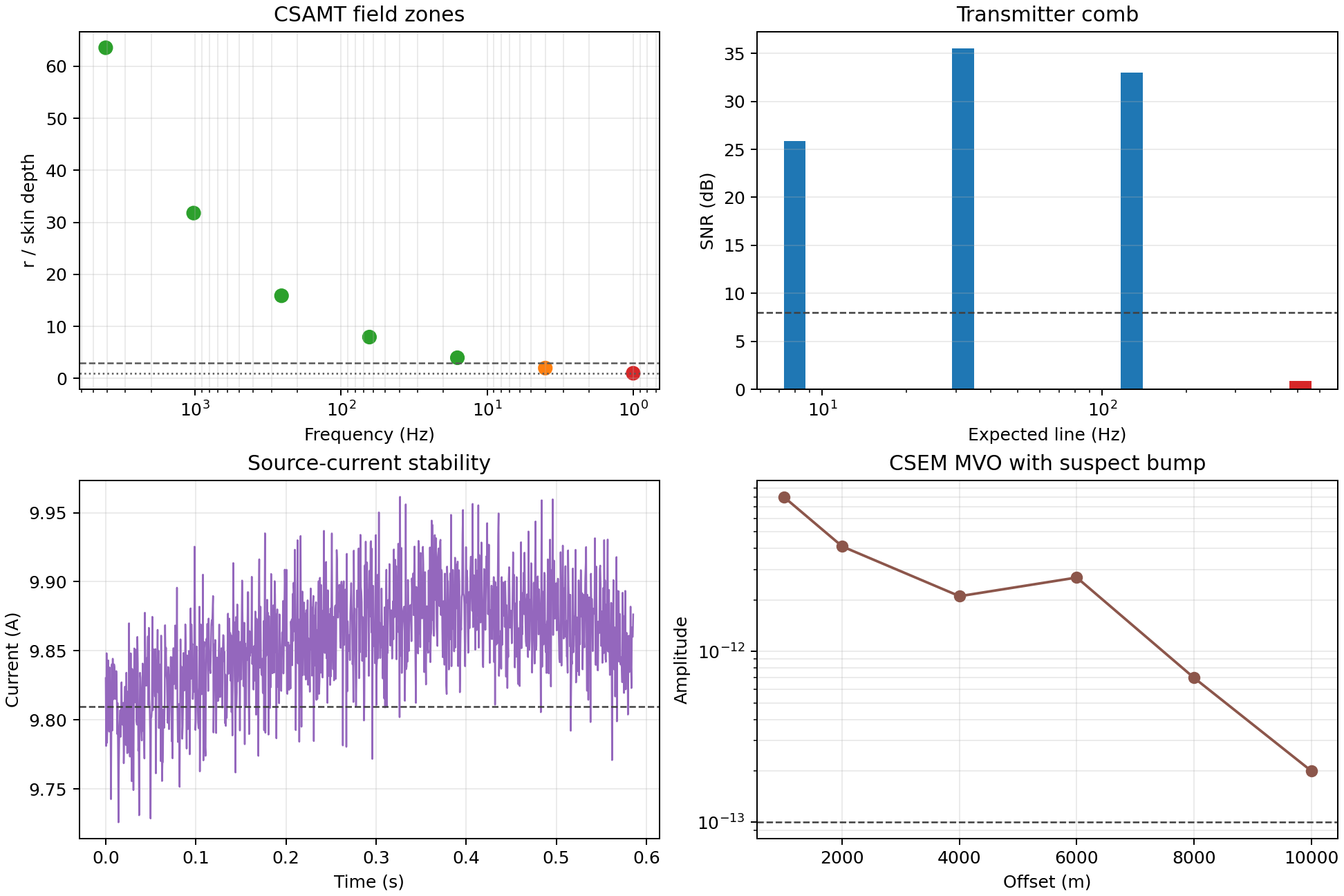
../../_images/user-guide-iot-controlled-source-01.png

The top-left panel plots the field-zone scatter on inverted log axes, so frequency decreases left to right, matching the direction skin depth grows. Five green points sit comfortably above the dashed far-field line at 3, the orange point sits between the two threshold lines in the transition band, and the red point sits at the bottom near a ratio of 1 — the same near/transition/far split already printed above, now visible as a shape rather than a table. The top-right panel’s three tall blue bars for 8, 32, and 128 Hz all clear the 8 dB dashed threshold with room to spare, while the missing 512 Hz line is a bar too short to see, coloured red. The bottom-left panel shows the source current oscillating around its mean (the dashed line at 9.81 A) with a visible slow upward drift over the first tenth of a second before settling — small enough that the CV stayed at 0.0066. The bottom-right panel is the clearest single picture on the page: an overall decay from \(10^{-11}\) to below \(10^{-13}\) amplitude over four orders of magnitude in offset, broken by one unmistakable uptick at 6000 m before the decay resumes — exactly the bump monotonic_decay: False flagged numerically.

9.4.10. Report Aggregation#

csamt_edge_report() and csem_edge_report() collate the per-channel diagnostics shown above into one dictionary each, and csamt_edge_table() / csem_edge_table() flatten one or more of those reports into pyCSAMT tables for multi-channel or multi-frequency reporting — the same table-building pattern amt_edge_table() uses on the natural-source side. In practice, keep the source packet, comb result, field-zone coverage, and CSEM offset response together in the field manifest so a later reviewer can see both the measured response and the source state that produced it. Method-Aware QC picks this up next, showing how a declared acquisition method gates which of these controlled-source checks even apply.