11.23. L-Curve Regularization Selection

pycsamt.emtools.lcurve helps choose a regularization parameter from a sweep of candidate models. Unlike most emtools pages, this module does not require EDI files or Sites objects. It only needs three arrays from a regularized inversion or smoothing experiment:

• data misfit, for example ||Gm - d||;

• model roughness, for example ||Lm||;

• optional regularization values, usually named lambda.

Full callable signatures live in the API reference. This page explains how to prepare the arrays, find the corner, plot the curve, compare methods, and turn the result into a reproducible report.

11.23.1. What The L-Curve Means

Regularization is a trade-off. A small regularization parameter usually fits the data more closely but allows a rough model. A large regularization parameter usually makes the model smoother but increases the data misfit.

In a standard Tikhonov problem the model \(m_\lambda\) is obtained by minimizing the objective function

\[\Phi_\lambda(m) = \|Gm - d\|_2^2 + \lambda^2\|Lm\|_2^2,\]

where \(G\) is the forward operator, \(d\) is the data vector, \(L\) is the roughness or damping operator, and \(\lambda\) controls how much roughness is penalized. The L-curve is built after solving this problem for many candidate values of \(\lambda\).

The L-curve plots these two quantities against each other:

\[x(\lambda) = \|Lm_\lambda\|_2, \qquad y(\lambda) = \|Gm_\lambda - d\|_2.\]

The useful value is often near the “corner” of the curve: the point where adding more smoothness begins to cost noticeably more data fit. That value is not magic, but it is a defensible starting point when you need to choose a regularization level from a sweep.

11.23.2. Inputs Expected By The Module

lcurve_table and plot_lcurve expect positive, finite arrays. Internally, non-finite and non-positive values are filtered out before log-scale calculations. The shortest valid array length controls the number of rows used.

The scoring is done in log-log space,

\[X_i = \log_{10} x_i, \qquad Y_i = \log_{10} y_i,\]

because the trade-off is usually multiplicative: a useful corner often means “this much extra smoothness costs this many times more misfit”, not a fixed additive change in raw units.

>>> import numpy as np
>>> lambdas = np.logspace(-3, 3, 60)
>>> roughness = 1.0 / (1.0 + lambdas**2)
>>> misfit = lambdas**2 / (1.0 + lambdas**2)
>>> # All three arrays should describe the same sweep order.
>>> assert misfit.shape == roughness.shape == lambdas.shape
>>> assert np.all(misfit > 0.0)
>>> assert np.all(roughness > 0.0)

The module does not compute the inversion itself. It only analyzes the numbers produced by your inversion, forward-model sweep, or smoothing experiment.

11.23.3. A Minimal Synthetic Example

Start with a curve whose corner is easy to see. This is useful for checking that the mechanics are clear before using real inversion output.

>>> from pycsamt.emtools import lcurve_table, plot_lcurve
>>> lambdas = np.logspace(-3, 3, 40)
>>> # Small lambda: rough model, low misfit.
>>> # Large lambda: smooth model, higher misfit.
>>> roughness = 1.0 / (1.0 + lambdas**2)
>>> misfit = lambdas**2 / (1.0 + lambdas**2)
>>> table = lcurve_table(misfit, roughness, lambdas)
>>> corner_idx = table.attrs["corner_idx"]
>>> table.iloc[corner_idx]
rough     0.412354
misfit    0.587646
lam       1.193777
curv      1.333709
slope    -0.711581
Name: 20, dtype: float64
>>> print("lambda* =", table["lam"].iloc[corner_idx])
lambda* = 1.1937766417144369
>>> ax = plot_lcurve(misfit, roughness, lambdas)
>>> ax.figure.savefig("synthetic_lcurve.png", dpi=200)

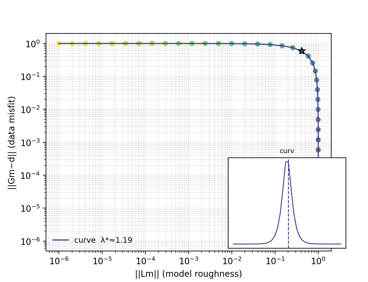
The returned table has columns rough, misfit, lam, curv, and slope. The selected row is stored separately as table.attrs["corner_idx"] so the table itself remains ordinary pandas data.

11.23.4. Read The Table

The table is the most important output because it lets you inspect the corner selection numerically.

>>> table = lcurve_table(
...     misfit,
...     roughness,
...     lambdas,
...     method="curvature",
...     smooth=3,
...     skip=1,
... )
>>> corner = table.attrs["corner_idx"]
>>> row = table.iloc[corner]
>>> print(f"corner index: {corner}")
corner index: 20
>>> print(f"lambda*: {row['lam']:.4g}")
lambda*: 1.194
>>> print(f"misfit: {row['misfit']:.4g}")
misfit: 0.5876
>>> print(f"roughness: {row['rough']:.4g}")
roughness: 0.4124
>>> print(f"corner score: {row['curv']:.4g}")
corner score: 1.334
>>> print(f"local slope: {row['slope']:.4g}")
local slope: -0.7116

curv is the corner score. With method="curvature", it is the numerical curvature of the log-log curve. With method="maxdist", it is the perpendicular distance from the line connecting the first and last log-log points.

For the curvature method, the score is the discrete version of

\[\kappa(t) = {|X'(t)Y''(t) - Y'(t)X''(t)| \over \left(X'(t)^2 + Y'(t)^2\right)^{3/2}},\]

where \(t\) is the ordered sweep index. The selected corner is the valid point with largest \(\kappa\).

11.23.5. Use A Dictionary Result

For small helper functions or serialization, return_dict=True gives arrays plus the selected corner index.

>>> from pycsamt.emtools import lcurve_table
>>> result = lcurve_table(
...     misfit,
...     roughness,
...     lambdas,
...     method="maxdist",
...     return_dict=True,
... )
>>> corner = result["corner"]
>>> lambda_star = result["lam"][corner]
>>> print(lambda_star)
0.8376776400682924

The dictionary keys are rough, misfit, lam, curv, slope, and corner.

11.23.6. Sorting And Sweep Order

The curve can be sorted by roughness, by lambda, or automatically. The default sort="auto" sorts by lambda when the lambda array is monotonic; otherwise it sorts by roughness.

>>> by_lambda = lcurve_table(
...     misfit,
...     roughness,
...     lambdas,
...     sort="lambda",
... )
>>> by_roughness = lcurve_table(
...     misfit,
...     roughness,
...     lambdas,
...     sort="x",
... )

Use sort="lambda" when you want to preserve the physical sweep direction. Use sort="x" when the lambda values are missing, duplicated, or not meaningful and the curve should simply be ordered from low to high roughness.

11.23.7. Corner Methods

Two corner-picking methods are available.

Method	How It Scores Points	When To Prefer It
"curvature"	Computes numerical curvature of the log-log curve.	Smooth, well-sampled curves.
"maxdist"	Finds the point farthest from the line joining the two endpoints.	Noisy curves, short sweeps, or uncertain smoothing.

>>> curvature = lcurve_table(
...     misfit,
...     roughness,
...     lambdas,
...     method="curvature",
...     smooth=3,
... )
>>> maxdist = lcurve_table(
...     misfit,
...     roughness,
...     lambdas,
...     method="maxdist",
... )
>>> j_curv = curvature.attrs["corner_idx"]
>>> j_dist = maxdist.attrs["corner_idx"]
>>> print("curvature lambda*:", curvature["lam"].iloc[j_curv])
curvature lambda*: 1.1937766417144369
>>> print("maxdist lambda*:", maxdist["lam"].iloc[j_dist])
maxdist lambda*: 0.8376776400682924

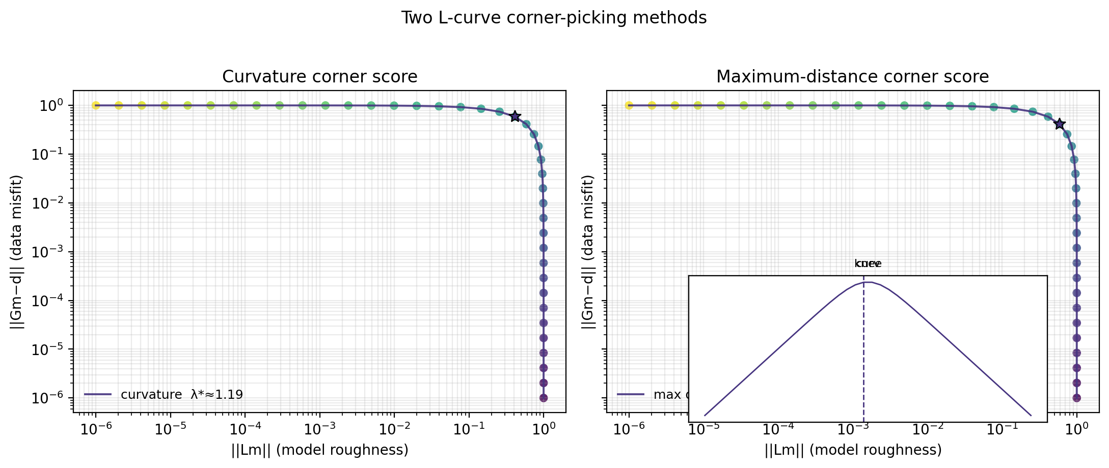
If the two methods choose similar values, the corner is probably stable. If they disagree strongly, inspect the curve and consider widening the lambda sweep.

The max-distance method works directly on the chord between the first and last log-log points. If \(\mathbf{p}_0=(X_0,Y_0)\) and \(\mathbf{p}_1=(X_n,Y_n)\), the score for point \(\mathbf{p}_i=(X_i,Y_i)\) is

\[d_i = {| (Y_n-Y_0)(X_i-X_0) - (X_n-X_0)(Y_i-Y_0) | \over \sqrt{(X_n-X_0)^2 + (Y_n-Y_0)^2}}.\]

This score is less sensitive to local numerical derivatives, which is why it is often a good cross-check for noisy or sparsely sampled sweeps.

11.23.8. Smoothing And Endpoint Skipping

The smooth argument affects the curvature method by applying a moving average in log-log space before differentiating. The skip argument prevents the first and last points from being selected as the corner.

>>> for smooth in (1, 3, 5, 7):
...     table = lcurve_table(
...         misfit,
...         roughness,
...         lambdas,
...         method="curvature",
...         smooth=smooth,
...         skip=2,
...     )
...     j = table.attrs["corner_idx"]
...     print(f"smooth={smooth}: lambda*={table['lam'].iloc[j]:.4g}")
...
smooth=1: lambda*=1.194
smooth=3: lambda*=1.194
smooth=5: lambda*=0.8377
smooth=7: lambda*=0.8377

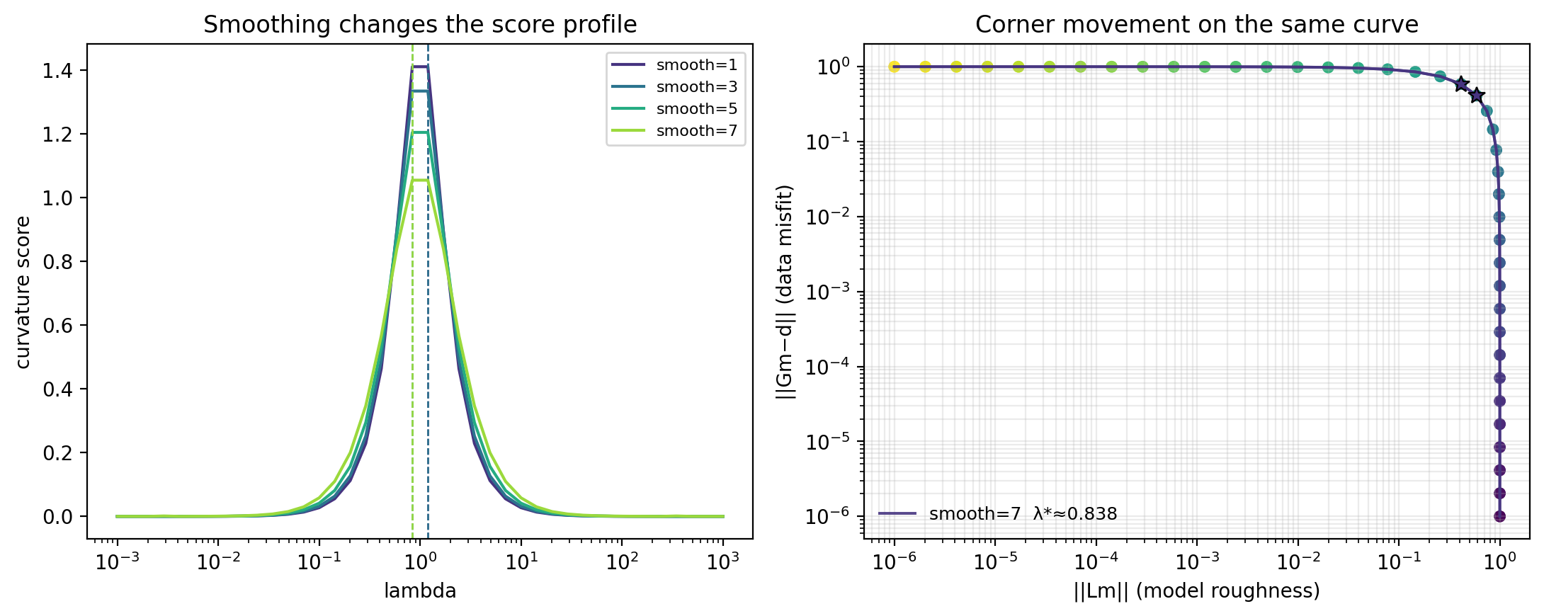
Be cautious with heavy smoothing. It can move the curvature maximum away from the visual corner, especially for short curves. maxdist is often a useful cross-check because it does not use numerical derivatives.

With smooth > 1, pyCSAMT applies a moving average to \(X_i=\log_{10}x_i\) and \(Y_i=\log_{10}y_i\) before computing derivatives:

\[\bar{X}_i = {1 \over w} \sum_{k=i-h}^{i+h} X_k, \qquad h = {w-1 \over 2}.\]

The same operation is applied to \(Y_i\). Smoothing is useful when the score curve is jagged, but it changes the curve being differentiated, so the selected \(\lambda^\ast\) should still be checked against the plotted model.

11.23.9. Plot A Single Curve

plot_lcurve draws roughness on the x-axis and misfit on the y-axis, both in log scale. The selected corner is marked with a star by default.

>>> import matplotlib.pyplot as plt
>>> fig, ax = plt.subplots(figsize=(6.4, 4.8))
>>> _ = plot_lcurve(
...     misfit,
...     roughness,
...     lambdas,
...     labels=["station 18-001A"],
...     method="curvature",
...     smooth=3,
...     show_inset=True,
...     ax=ax,
... )
>>> _ = ax.set_title("L-curve regularization sweep")
>>> fig.tight_layout()
>>> fig.savefig("lcurve_18-001A.png", dpi=200)

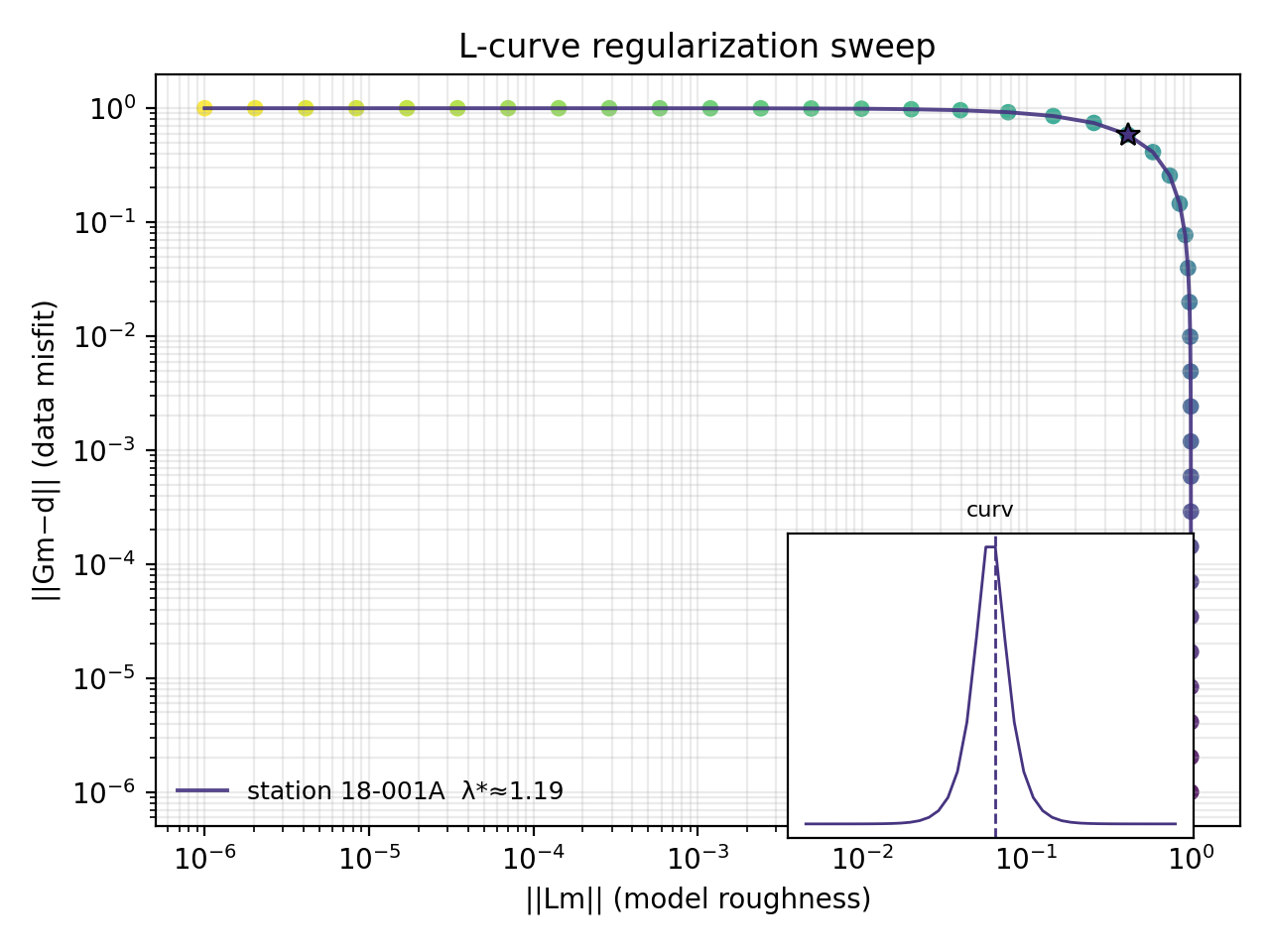
The inset shows the corner score. For method="curvature" the inset title is curv. For method="maxdist" it is knee.

11.23.10. Plot Multiple Curves

Pass lists of misfit, roughness, and lambda arrays to compare several stations, inversion targets, or model parameterizations.

>>> curves_misfit = [
...     misfit,
...     misfit * 1.25 + 0.03,
...     misfit * 0.85 + 0.08,
... ]
>>> curves_roughness = [
...     roughness,
...     roughness * 0.75 + 0.02,
...     roughness * 1.35 + 0.05,
... ]
>>> curves_lambda = [lambdas, lambdas, lambdas]
>>> fig, ax = plt.subplots(figsize=(7.0, 5.0))
>>> _ = plot_lcurve(
...     curves_misfit,
...     curves_roughness,
...     curves_lambda,
...     labels=["run A", "run B", "run C"],
...     method="maxdist",
...     show_inset=True,
...     ax=ax,
... )
>>> fig.savefig("lcurve_multi_run.png", dpi=200)

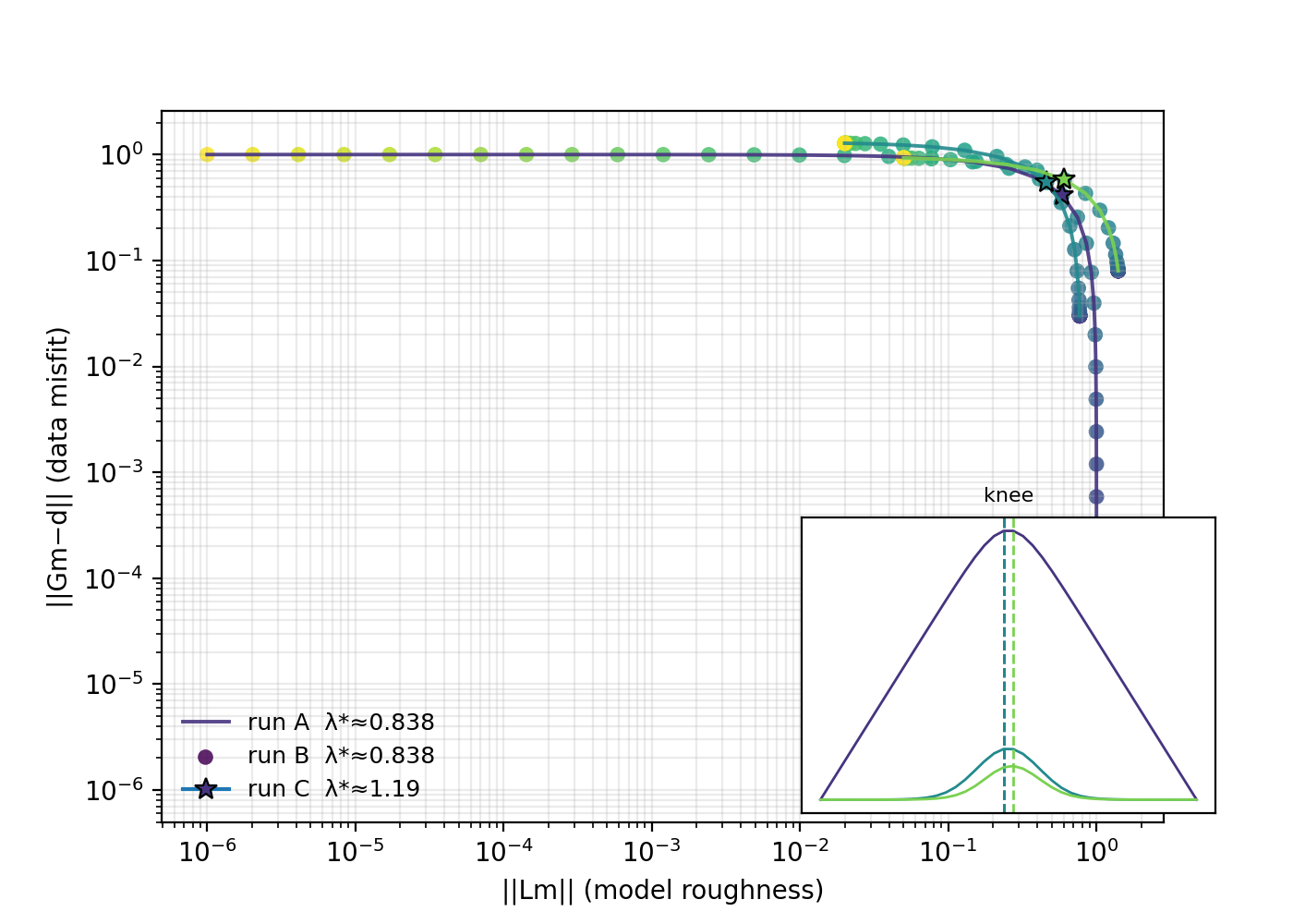
The plot uses one shared inset for all curves, so the corner scores can be compared in the same small panel. The legend reports the selected lambda* for each curve when lambda values are supplied.

11.23.11. Show Sweep Direction

arrow_every draws arrows along the curve. This is helpful when you want readers to see how increasing lambda moves through the trade-off.

>>> ax = plot_lcurve(
...     misfit,
...     roughness,
...     lambdas,
...     arrow_every=5,
...     show_points=False,
...     show_inset=False,
... )
>>> ax.figure.savefig("lcurve_with_lambda_direction.png", dpi=200)

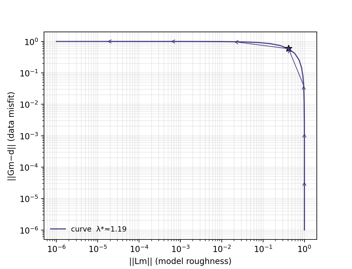
Use arrows when teaching or reviewing a sweep. For compact reports, points plus the corner marker are usually enough.

11.23.12. Use L-Curve With A Real Smoothing Sweep

The example below builds a small Tikhonov smoothing problem from one station’s apparent resistivity. It is not a full inversion; it is a transparent way to produce real misfit and roughness arrays.

The model vector is the smoothed \(\log_{10}\rho_a(T)\) curve. The second-difference operator is

\[(Dm)_i = m_i - 2m_{i+1} + m_{i+2},\]

so \(\|Dm\|_2\) penalizes curvature in the sounding rather than its absolute level. For this simple smoothing problem, the normal equation is

\[(I + \lambda^2 D^T D)m_\lambda = d.\]

>>> from pycsamt.emtools import ensure_sites
>>> from pycsamt.emtools._core import _get_z_block, _iter_items, _name
>>> survey = ensure_sites("data/AMT/WILLY_DATA/L18PLT", strict=True)
>>> def second_difference(n):
...     operator = np.zeros((n - 2, n))
...     for i in range(n - 2):
...         operator[i, i] = 1.0
...         operator[i, i + 1] = -2.0
...         operator[i, i + 2] = 1.0
...     return operator
...
>>> def station_log10_rho_xy(sites, station):
...     for index, site in enumerate(_iter_items(sites)):
...         if _name(site, index) != station:
...             continue
...         _, z, freq = _get_z_block(site)
...         rho_xy = 0.2 * np.abs(z[:, 0, 1]) ** 2 / freq
...         return np.log10(rho_xy), freq
...     raise KeyError(station)
...
>>> def smoothing_sweep(data, lambdas):
...     n = data.size
...     identity = np.eye(n)
...     rough_operator = second_difference(n)
...     regularizer = rough_operator.T @ rough_operator
...     misfits = []
...     roughness = []
...     models = []
...     for lam in lambdas:
...         model = np.linalg.solve(
...             identity + lam**2 * regularizer,
...             data,
...         )
...         misfits.append(np.linalg.norm(model - data))
...         roughness.append(np.linalg.norm(rough_operator @ model))
...         models.append(model)
...     return np.array(misfits), np.array(roughness), np.array(models)
...
>>> lambdas = np.logspace(-3, 3, 60)
>>> data, freq = station_log10_rho_xy(survey, "18-001A")
>>> misfit, roughness, models = smoothing_sweep(data, lambdas)
>>> table = lcurve_table(misfit, roughness, lambdas)
>>> corner = table.attrs["corner_idx"]
>>> print("lambda* =", table["lam"].iloc[corner])
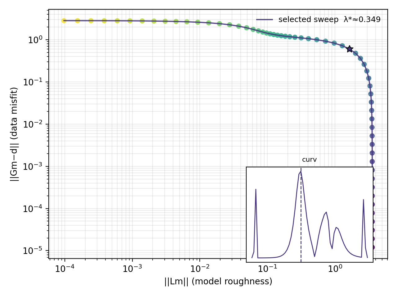
lambda* = 0.34863652276780877
>>> ax = plot_lcurve(misfit, roughness, lambdas, labels=["18-001A"])
>>> ax.figure.savefig("lcurve_real_station.png", dpi=200)

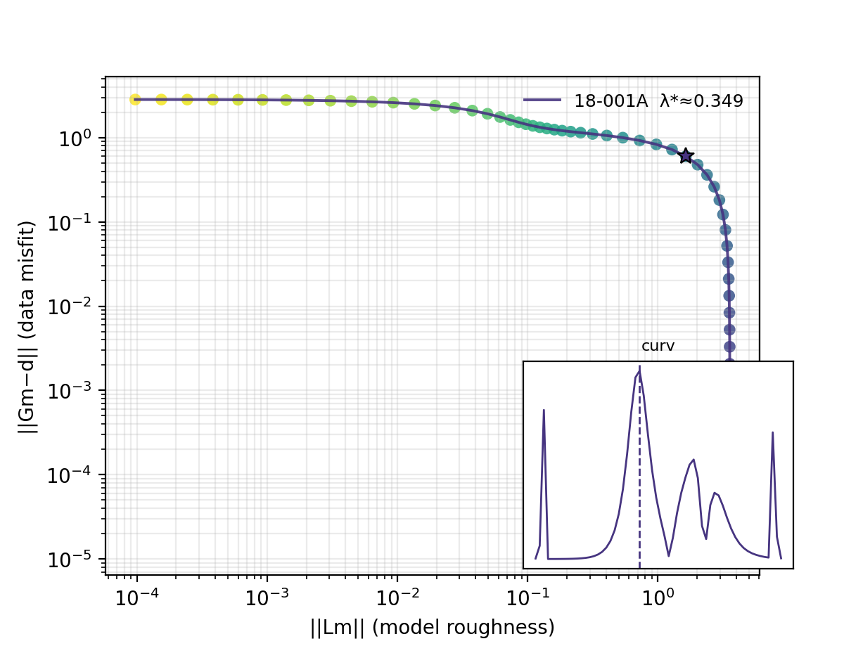
This code makes the L-curve inputs explicit. misfit measures how far the smoothed model is from the observed log-resistivity curve. roughness measures how curved the smoothed model remains after applying the second-difference operator.

The important part is not that this is a full inversion; it is that the arrays passed to lcurve_table come from a real regularized solve. In production you would replace this small smoothing system with the misfit and roughness reported by your inversion engine.

11.23.13. Inspect What Lambda Does

After choosing a corner, plot the model at the corner against clearly under- and over-regularized choices. This is the best sanity check.

For a small \(\lambda\), the term \(\|Gm-d\|_2^2\) dominates and the model follows the data closely. For a large \(\lambda\), the roughness penalty dominates and the model approaches the smoothest curve allowed by \(L\). The corner is useful only if the model at \(\lambda^\ast\) is a credible compromise between those two behaviors.

>>> period = 1.0 / freq
>>> corner = table.attrs["corner_idx"]
>>> under = 5
>>> over = 50
>>> fig, ax = plt.subplots(figsize=(7.0, 4.5))
>>> _ = ax.semilogx(period, data, "o", color="0.55", label="observed")
>>> _ = ax.semilogx(
...     period,
...     models[under],
...     "-",
...     label=f"under-regularized lambda={lambdas[under]:.3g}",
... )
>>> _ = ax.semilogx(
...     period,
...     models[corner],
...     "-",
...     linewidth=2.2,
...     label=f"corner lambda={lambdas[corner]:.3g}",
... )
>>> _ = ax.semilogx(
...     period,
...     models[over],
...     "-",
...     label=f"over-regularized lambda={lambdas[over]:.3g}",
... )
>>> _ = ax.set_xlabel("Period (s)")
>>> _ = ax.set_ylabel("log10 apparent resistivity")
>>> _ = ax.legend(fontsize=8)
>>> fig.savefig("regularization_levels.png", dpi=200)

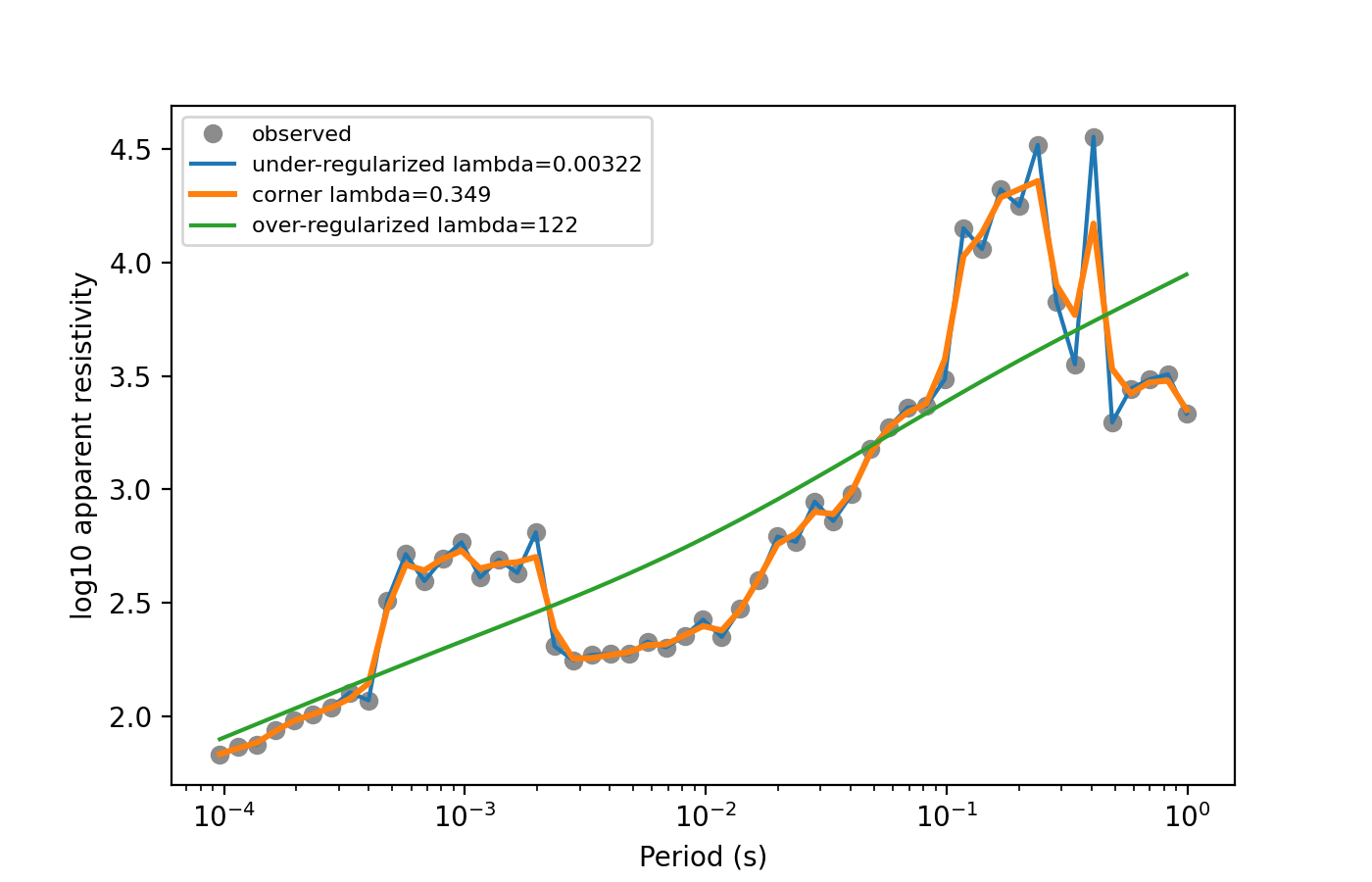
The under-regularized model should usually track too much local noise. The over-regularized model should usually be too smooth. The corner model should sit between them.

11.23.14. Reading Real Inversion Logs

The smoothing sweep above builds misfit/roughness/lambda arrays by hand. Real 2-D and 3-D inversion codes already write exactly these three quantities to their convergence logs, one row per iteration, because Occam-style regularized inversion is an L-curve sweep: each iteration searches for the regularization parameter that best trades data fit against model roughness, then moves on. Three loader functions read those logs directly into an LCurveData container, so the same lcurve_table() and plot_lcurve() used throughout this page work unchanged on real solver output:

Function	Reads	Regularization parameter
lcurve_from_occam2d	Occam2D’s LogFile.logfile	Accepted Lagrange multiplier \(\mu\) (linear scale).
lcurve_from_modem	ModEM’s Modular_NLCG.log	Damping parameter \(\lambda\) (linear scale).
lcurve_from_mare2dem	MARE2DEM’s *.logfile	Optimal \(\mu\), converted from the log’s \(\log_{10}\mu\) back to linear scale.

Each function delegates to the existing, already-tested log parser for that backend (OccamLog, ModEmLog, Mare2DEMLog) rather than re-parsing the log text, and drops any row whose misfit or roughness is non-finite or non-positive – for example an Occam2D iteration that stopped on “Convergence problems” before writing ROUGHNESS IS, or a ModEM START record whose model-norm term m2 is exactly zero before the first iteration.

11.23.14.1. Occam2D

>>> from pycsamt.emtools import lcurve_from_occam2d
>>> occam_sweep = lcurve_from_occam2d("data/occam2D/LogFile.logfile")
>>> occam_sweep.backend
'occam2d'
>>> occam_sweep.misfit.size
16
>>> ax = occam_sweep.plot(
...     method="curvature",
...     smooth=3,
...     show_inset=False,
...     target_misfit=1.0,
...     target_label="target RMS = 1.0",
...     label_every=4,
...     label_prefix="mu=",
...     figsize=(7.5, 5.2),
... )
>>> _ = ax.set_title("Occam2D real inversion L-curve (data/occam2D)")
>>> ax.figure.tight_layout()
>>> ax.figure.savefig("occam2d_lcurve.png", dpi=170)

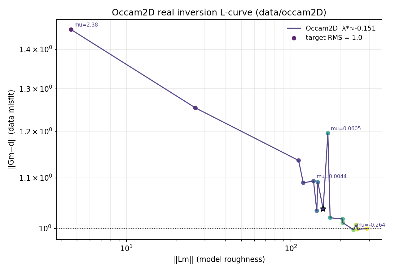
Sixteen of the seventeen logged iterations survive filtering (the seventeenth never finishes writing ROUGHNESS IS – the log ends with “Convergence problems from RMS Misfit” instead). Occam’s own search variable \(\mu\) is not the linear \(\lambda\) used earlier in this page; it behaves closer to \(\log_{10}\lambda\) and can go negative, which is exactly what the mu= labels on the plot show happening once the run crosses the target RMS. The curve itself is not a clean textbook L: real Occam runs cut step size and re-search \(\mu\) whenever a step overshoots, which shows up here as the visible zig-zag once roughness passes about 150.

11.23.14.2. ModEM

>>> from pycsamt.emtools import lcurve_from_modem
>>> modem_sweep = lcurve_from_modem(
...     "data/modem/willy_27freq_watex_line02_sample/Modular_NLCG.log"
... )
>>> modem_sweep.backend
'modem'
>>> modem_sweep.misfit.size
73
>>> ax = modem_sweep.plot(
...     method="curvature",
...     smooth=3,
...     show_inset=False,
...     target_misfit=1.05,
...     target_label="exit RMS = 1.05",
...     label_every=12,
...     label_prefix="lam=",
...     figsize=(7.5, 5.2),
... )
>>> _ = ax.set_title("ModEM real NLCG inversion L-curve (willy_27freq_watex_line02)")
>>> ax.figure.tight_layout()
>>> ax.figure.savefig("modem_lcurve.png", dpi=170)

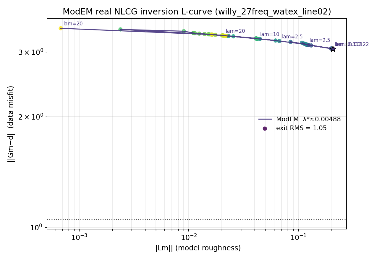
ModEM’s roughness axis is its model-regularization term m2 – lcurve_from_modem() passes it straight through as rough, since it plays the identical \(\Phi_m(m)\) role that Occam’s ROUGHNESS IS plays. The bundled sample’s own inv.ctrl sets Exit search when rms is less than 1.05, plotted here as the target line; 73 NLCG iterations still leave the run at RMS ≈ 3.06, far short of it. That is not a bug in the reader – it is an honest read of a deliberately compact bundled sample, not a converged production inversion, and the target line makes that gap visible at a glance instead of hiding it in an axis range that only covers the data.

11.23.14.3. MARE2DEM

>>> from pycsamt.emtools import lcurve_from_mare2dem
>>> mare_sweep = lcurve_from_mare2dem(
...     "data/mare2dem/demo_mt_inversion/demo.logfile"
... )
>>> mare_sweep.backend
'mare2dem'
>>> mare_sweep.misfit.size
6
>>> ax = mare_sweep.plot(
...     method="curvature",
...     smooth=3,
...     show_inset=False,
...     target_misfit=1.0,
...     target_label="target misfit = 1.0",
...     label_every=1,
...     label_prefix="mu=",
...     figsize=(7.5, 5.2),
... )
>>> _ = ax.set_title("MARE2DEM real MT inversion L-curve (demo_mt_inversion)")
>>> ax.figure.tight_layout()
>>> ax.figure.savefig("mare2dem_lcurve.png", dpi=170)

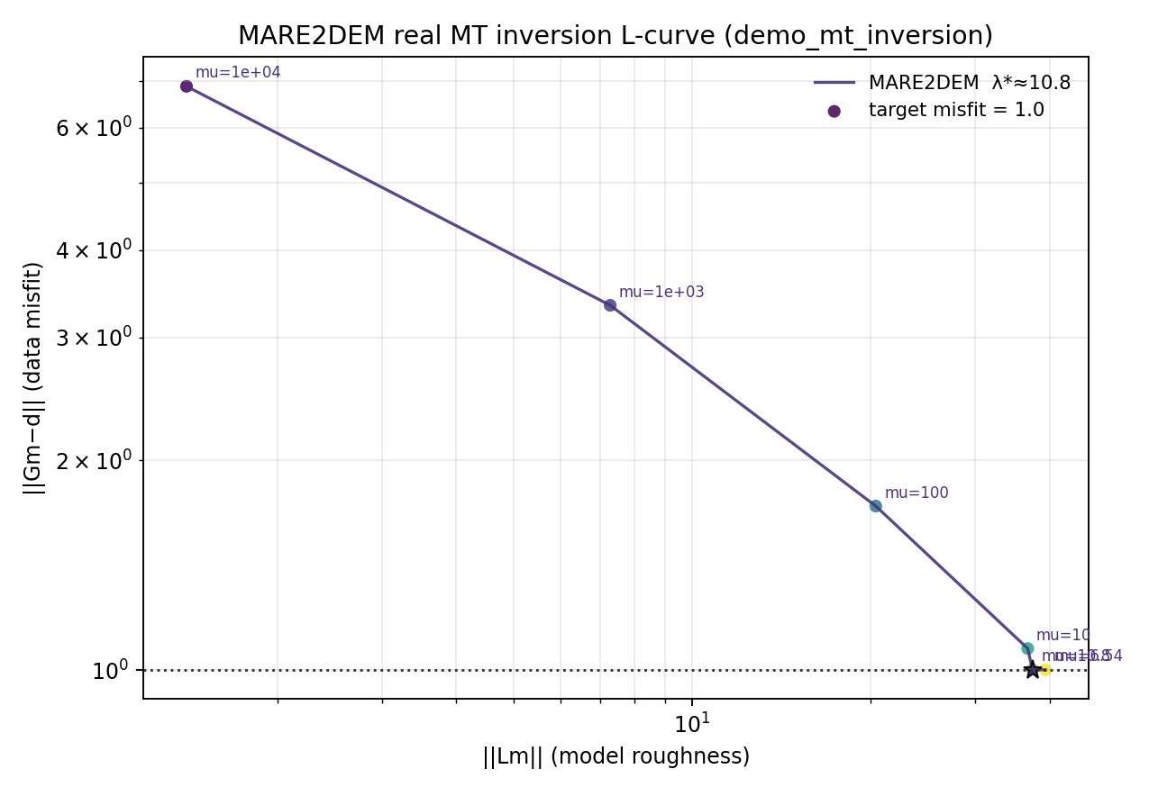
MARE2DEM logs only six completed iterations for this bundled MT demo, and it reaches the target misfit by iteration 5 – close enough that iteration 6 actually overshoots slightly (misfit rises from 1.001 to 1.002) as the mu search steps past the target. With only six points the curvature and max-distance corner scores have little to work with, so treat the corner pick on a sweep this short as a rough guide, not a precise answer.

11.23.15. Compare Corner Methods On Real Data

The “Curvature and max-distance disagree” failure mode described below is not hypothetical – it shows up on all three real logs above, and by very different margins.

>>> import pandas as pd
>>> rows = []
>>> for name, sweep in [
...     ("occam2d", occam_sweep),
...     ("modem", modem_sweep),
...     ("mare2dem", mare_sweep),
... ]:
...     tc = sweep.table(method="curvature")
...     tm = sweep.table(method="maxdist")
...     jc, jm = tc.attrs["corner_idx"], tm.attrs["corner_idx"]
...     rows.append(
...         {
...             "backend": name,
...             "n_iter": sweep.misfit.size,
...             "curv_misfit": tc["misfit"].iloc[jc],
...             "curv_rough": tc["rough"].iloc[jc],
...             "maxdist_misfit": tm["misfit"].iloc[jm],
...             "maxdist_rough": tm["rough"].iloc[jm],
...         }
...     )
...
>>> summary = pd.DataFrame(rows)
>>> print(summary.to_string(index=False))
 backend  n_iter  curv_misfit  curv_rough  maxdist_misfit  maxdist_rough
 occam2d      16     1.037446  157.348700        1.195972     168.152600
   modem      73     3.057482    0.206766        3.417263       0.008998
mare2dem       6     1.002000   37.440000        3.336000       7.278000

Occam2D’s two methods land close together (roughness 157 vs. 168 – both describe the same tight zig-zag near the target). ModEM’s do not: curvature settles on the very last, flattest part of the sweep (roughness ≈ 0.21) while max-distance picks a point two decades rougher-tolerant near the start of the run (roughness ≈ 0.009) – exactly the instability the smoothing-and-endpoint-skipping section above warns about on a noisy, non-monotonic real curve. MARE2DEM’s six points are too few for either score to be more than a rough pointer. When the two methods disagree this much, prefer the plotted curve and domain knowledge (a target misfit, a known noise floor) over either automatic corner pick.

11.23.16. Common Failure Modes

Corner at the first or last lambda

The sweep probably does not bracket the useful region. Extend the lambda range and rerun the sweep. Increasing skip can hide the endpoint, but it cannot fix a badly chosen sweep.

Misfit or roughness contains zeros

Log-scale L-curve scoring requires positive values. The module filters non-positive values, but you should still investigate why they occurred.

Curvature and max-distance disagree

The curve may be noisy, too short, too heavily smoothed, or not truly L-shaped. Plot both methods and inspect the model curves at both selected lambdas.

Multiple curves have very different scales

That can be normal when stations or inversions differ strongly. Compare selected lambdas and model behavior, not only absolute misfit and roughness values.

The curve is nearly a straight line

There may not be a meaningful trade-off in the swept range. Try a wider lambda interval or revisit the definition of misfit and roughness.

11.23.17. Save A Reproducible L-Curve Bundle

This script writes the table, selected corner, plot, and a short text summary for one sweep.

>>> from pathlib import Path
>>> out = Path("lcurve_report")
>>> out.mkdir(parents=True, exist_ok=True)
>>> table = lcurve_table(
...     misfit,
...     roughness,
...     lambdas,
...     method="curvature",
...     smooth=3,
...     skip=1,
... )
>>> corner = table.attrs["corner_idx"]
>>> table.to_csv(out / "lcurve_table.csv", index=False)
>>> corner_row = table.iloc[corner]
>>> with (out / "corner.txt").open("w", encoding="utf-8") as stream:
...     stream.write(f"corner_index: {corner}\n")
...     stream.write(f"lambda_star: {corner_row['lam']:.8g}\n")
...     stream.write(f"misfit: {corner_row['misfit']:.8g}\n")
...     stream.write(f"roughness: {corner_row['rough']:.8g}\n")
...     stream.write(f"score: {corner_row['curv']:.8g}\n")
...
17
24
19
20
17
>>> fig, ax = plt.subplots(figsize=(6.4, 4.8))
>>> _ = plot_lcurve(
...     misfit,
...     roughness,
...     lambdas,
...     labels=["selected sweep"],
...     method="curvature",
...     smooth=3,
...     ax=ax,
... )
>>> fig.tight_layout()
>>> fig.savefig(out / "lcurve.png", dpi=200)

11.23.18. Worked Example

The gallery example builds a real regularization sweep from bundled apparent-resistivity data and compares corner-picking methods.

Open the rendered gallery page here: L-curve regularization-parameter selection (pycsamt.emtools.lcurve).