
11.18. Source Effects And Near-Field Correction#
pycsamt.emtools.source_effects helps diagnose when the artificial
CSAMT transmitter is influencing the measured response. Natural-source
MT interpretation assumes a plane-wave source. CSAMT does not have that
luxury: the transmitter has a finite offset from each receiver, and the
offset can control whether a station-frequency row behaves like
near field, transition field, or far field.
The module contains two related but independent families of tools:
Yan and Fu / Da et al. source overprint diagnostics, based on the ground-wave to surface-wave amplitude ratio \(\beta_{Ey}\).
Wang and Lin normalized-response and near-field correction tools, based on skin-depth field zones and an equatorial horizontal electric dipole correction factor.
Full function signatures and parameter defaults are maintained in the
API reference. This guide uses the public
two-level imports from pycsamt.emtools. Every example below uses
pyCSAMT’s bundled data/CSAMT line – real
grounded dipole transmitter data from a groundwater-exploration
survey in the Tongkeng area, Hunan Province, China (Kouadio et al.,
2020) [Kouadio2020], the same ten-station line examined in
CSAMT Field-Zone Classification. Unlike the natural-source AMT/MT lines used
elsewhere in emtools, this survey genuinely has a controlled-source
transmitter and a real offset, so the diagnostics on this page are
measuring something that actually exists in the data, not a synthetic
what-if.
11.18.1. Why Offset Matters#
Every source-effect calculation needs a source-receiver offset r.
Standard EDI files usually do not store the CSAMT transmitter geometry,
so you must provide the offset explicitly unless your station objects
already carry an attribute such as source_offset, offset, or
dist. The Tongkeng field notes place the transmitter at roughly
1 km from the line, so this page uses source_offset=1000.0 as its
scalar default and, in the closing sections, a small per-station
transmitter-receiver offset dictionary:
>>> source_offset = 1000.0
>>> source_offset_by_station = {
...     "csa000": 950.0,
...     "csa050": 975.0,
...     "csa100": 1000.0,
... }
Use a scalar only when the same representative offset is justified for all stations. For field processing, prefer a station dictionary derived from transmitter and receiver coordinates – exactly the pattern used in CSAMT Field-Zone Classification for the same survey.
11.18.2. Workflow Map#
Goal |
Use this |
Output |
|---|---|---|
Evaluate pure overprint beta |
|
\(\beta_{Ey}\) in percent for arrays or scalars. |
Build per-frequency overprint table |
|
Long-form table with |
Summarize overprint by station |
|
Station table with max/mean beta, fraction flagged, and slopes. |
Plot beta pseudo-section |
|
Station-period map of \(\beta_{Ey}\). |
Normalize response |
|
Apparent-resistivity ratio, phase residual, field zone, and |
Correct near-field response |
|
|
Plot normalized response |
|
Two-panel pseudo-section of normalized resistivity and phase. |
11.18.3. Loading A Survey#
Load the survey once with ensure_sites. Keep the raw object unchanged
while you inspect source effects and test correction settings.
>>> from pycsamt.emtools import ensure_sites
>>> sites = ensure_sites("data/CSAMT", recursive=False, strict=True)
>>> len(list(sites))
10
Ten stations, csa000 through csa450, each with 17 frequencies –
170 station-frequency rows in total for every table below. Every EDI in
this survey records only the Zxy component (scalar single-dipole
CSAMT); the functions on this page fall back to it automatically
wherever a determinant-style quantity would otherwise need both
off-diagonal components.
11.18.4. Overprint Beta#
overprint_beta is the pure mathematical interface. It does not need
EDI files. It evaluates the Yan and Fu ground-wave to surface-wave ratio
and returns \(\beta_{Ey}\) in percent. In this workflow,
source overprint means the finite transmitter contribution is
large enough to bias a plane-wave interpretation.
The measured field at the receiver is the sum of a ground wave that travels directly through the earth from the source and a surface wave guided along the air-earth interface; a plane-wave (natural-source MT) interpretation is only valid once the ground wave dominates. Yan & Fu (2004, eq. 6) quantify that balance as the ratio of how sharply each term varies near the receiver:
where \(P\) is the Sommerfeld ground-wave term, \(r_3\) is the
3-D distance from the dipole source to the evaluation point, \(N\)
is the Foster surface-wave term built from modified Bessel functions
\(I_0\) and \(K_0\), and \(k_1 = \sqrt{i\omega\mu_0/\rho}\)
is the complex earth wavenumber. overprint_beta evaluates the
required partial derivatives by central finite differences rather than
a closed-form expression, which is why it needs a half-space
resistivity, not just an offset – the same offset can sit deep in the
near field over resistive ground and comfortably in the far field over
conductive ground.
>>> import numpy as np
>>> from pycsamt.emtools import BETA_THRESH_PCT, overprint_beta
>>> freq = np.logspace(-1, 3, 60)
>>> rho = 1170.0
>>> for offset in (500.0, 1000.0, 4000.0):
...     beta_pct = overprint_beta(rho=rho, freq=freq, offset=offset)
...     contaminated = freq[beta_pct > BETA_THRESH_PCT]
...     if contaminated.size:
...         print(
...             f"offset={offset:g} m: beta>{BETA_THRESH_PCT:g}% "
...             f"up to {contaminated.max():.3g} Hz"
...         )
...     else:
...         print(f"offset={offset:g} m: beta never exceeds {BETA_THRESH_PCT:g}%")
...
offset=500 m: beta>3% up to 1e+03 Hz
offset=1000 m: beta>3% up to 1e+03 Hz
offset=4000 m: beta>3% up to 392 Hz
rho = 1170 \(\Omega\cdot\mathrm{m}\) here is not an arbitrary
round number: it is the median apparent resistivity across this exact
survey’s far-field-classified rows, the same value derived from
CSAMT Field-Zone Classification’s field-zone classification and reused again
in Phased-Array Source Design. At both the 500 m and 1000 m offsets –
straddling this survey’s real ~1 km transmitter distance – beta stays
above the 3 percent threshold across the entire swept band, up to the
top of the sweep at 1000 Hz. Only pulling the offset out to 4000 m
brings the contaminated range down to below 392 Hz. BETA_THRESH_PCT
is 3.0. Values above that threshold indicate potential source
overprint under the Yan and Fu criterion. The threshold is useful, but
the exact result depends strongly on rho, frequency, and offset.
11.18.5. Per-Frequency Overprint Detection#
detect_source_overprint applies overprint_beta to every
station-frequency row using apparent resistivity computed from the
observed impedance tensor. Alongside beta_pct, it reports kr,
a dimensionless field-zone parameter that recurs throughout this page:
the source-receiver offset measured in Bostick skin depths at that
frequency. Small kr means the offset is well inside one skin depth
– the near field, where beta_pct is expected to be large – while
large kr means the offset is many skin depths away, deep in the far
field where beta_pct should be small.
>>> from pycsamt.emtools import detect_source_overprint
>>> detail = detect_source_overprint(
...     sites,
...     source_offset=1000.0,
...     beta_threshold=3.0,
... )
>>> detail.head()
  station    freq_hz  period_s  ...         kr   beta_pct  overprint_flag
0  csa000  8196.7220  0.000122  ...  15.285344   0.016192           False
1  csa000  4098.3610  0.000244  ...   6.542431   3.566184            True
2  csa000  2049.1800  0.000488  ...   2.957325  23.053786            True
3  csa000  1023.5410  0.000977  ...   1.378964  41.538102            True
4  csa000   512.8206  0.001950  ...   0.988957  45.657295            True

[5 rows x 8 columns]
>>> detail["beta_pct"].describe()
count    170.000000
mean      42.677668
std       14.419220
min        0.016192
25%       45.357665
50%       49.994890
75%       49.999936
max       50.000025
Name: beta_pct, dtype: float64
>>> detail["overprint_flag"].value_counts()
overprint_flag
True     162
False      8
Name: count, dtype: int64
The returned table has one row per station and frequency:
station, freq_hz, period_s, offset_m, rho_a_ohmm,
kr, beta_pct, overprint_flag
Rows with unknown offset keep the station and frequency information, but
kr and beta_pct are NaN. That is intentional: source-effect
diagnostics cannot be inferred honestly without geometry. On this real
line, 162 of 170 station-frequency rows – 95 percent – are flagged.
csa000’s own progression from the table above tells the story
plainly: kr starts at 15.3 at the highest frequency, where beta
is a negligible 0.02 percent, and collapses toward 1 as
frequency drops, where beta saturates near its 50 percent ceiling.
The median across the whole survey, 49.99 percent, sits right at
that same ceiling – this transmitter offset was simply too short for
most of this line’s frequency band.
11.18.6. Station-Level Summary#
source_overprint_table summarizes the long-form table by station. It
adds maximum and mean \(\beta\), the number and fraction of flagged
rows, and a low-/high-frequency slope comparison inspired by Da et al.
(2016). f_split splits each station’s rows into a low-frequency and
a high-frequency group, and each group gets its own ordinary
least-squares slope of log-apparent-resistivity against log-frequency:
A source sitting over a resistive body radiates differently than one
over a conductor, and that difference shows up as a change in slope
between the two bands rather than as a single anomalous value – a
strongly negative slope_delta (low-frequency slope much shallower
than high-frequency slope) is the Da et al. signature of a resistivity
contrast beneath the source dipole itself, distinct from a genuine
subsurface target under the receiver.
>>> from pycsamt.emtools import source_overprint_table
>>> summary = source_overprint_table(
...     sites,
...     source_offset=1000.0,
...     beta_threshold=3.0,
...     f_split=50.0,
... )
>>> cols = [
...     "station",
...     "beta_max_pct",
...     "beta_mean_pct",
...     "n_overprint",
...     "overprint_frac",
...     "lf_slope",
...     "hf_slope",
...     "slope_delta",
...     "overprint_flag",
... ]
>>> summary[cols].sort_values("overprint_frac", ascending=False).head()
  station  beta_max_pct  beta_mean_pct  ...  hf_slope  slope_delta  overprint_flag
4  csa200     49.999981      41.818166  ... -0.339186    -0.632794            True
5  csa250     50.000025      43.946283  ... -0.384489    -0.559169            True
0  csa000     49.999981      41.914951  ... -0.893507    -0.055431            True
1  csa050     50.000025      43.071339  ... -0.568374    -0.390639            True
2  csa100     50.000003      42.759419  ... -0.679451    -0.263436            True

[5 rows x 9 columns]
f_split separates low- and high-frequency bands for slope analysis.
Choose it from the actual survey frequency range – 50 Hz sits
comfortably inside this line’s real 0.125-8196.722 Hz band. If the
split falls outside the sampled range, one of the slope columns will be
NaN.
11.18.7. Overprint Pseudo-Section#
plot_overprint_section maps \(\beta_{Ey}\) across station and
period. It can contour key beta levels, including the 3 percent
threshold.
>>> import matplotlib.pyplot as plt
>>> from pycsamt.emtools import plot_overprint_section
>>> fig, ax = plt.subplots(figsize=(10, 5))
>>> _ = plot_overprint_section(
...     sites,
...     source_offset=1000.0,
...     beta_threshold=3.0,
...     beta_levels=(1.0, 3.0, 10.0, 30.0),
...     period_axis=True,
...     log_y=True,
...     ax=ax,
... )
>>> fig.tight_layout()
>>> fig.savefig("source_overprint_section_csamt.png", dpi=200)
>>> plt.close(fig)
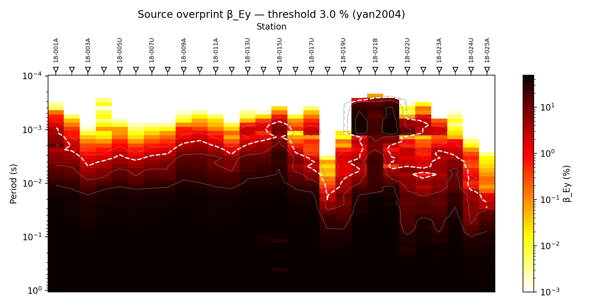
Nearly the entire pseudo-section is saturated near-black – the deepest
colour on this scale – across every period longer than about
\(2\times10^{-3}\) s. Only the shortest-period row at the very top
shows real station-to-station variation, from pale yellow (csa350,
essentially unflagged) through orange to saturated red. If most of the
plot sits above the threshold, as it does here, the assumed offset may
place much of the survey outside a clean far-field regime – exactly
what the 95 percent flagged-row count above already showed numerically.
11.18.8. Normalized Response#
normalize_response implements the Wang and Lin view of source
effects. It computes:
It also classifies each row using the skin depth relation \(\delta = 503\sqrt{\rho_a/f}\) and the source offset:
nearwhenr / delta < 0.5(near field);transitionwhen0.5 <= r / delta < 4(transition field);farwhenr / delta >= 4(far field).
This 503-based skin depth and the classic near/transition/far bands are
Wang and Lin’s own criterion, a different (stricter, and differently
scaled) rule from CSAMT Field-Zone Classification’s Bostick-depth-based
|kr| thresholds – the two pages should not be expected to draw the
near/far boundary at exactly the same frequency for the same station,
only to agree on the broad picture.
>>> from pycsamt.emtools import normalize_response
>>> norm = normalize_response(
...     sites,
...     rho_ref=1170.0,
...     source_offset=1000.0,
...     comp="det",
...     phi_ref_deg=45.0,
... )
>>> norm.head()
  station    freq_hz  period_s  ...  phi_diff_deg        zone         kr
0  csa000  8196.7220  0.000122  ...    -78.300008         far  10.814648
1  csa000  4098.3610  0.000244  ...    -57.200000         far   4.628884
2  csa000  2049.1800  0.000488  ...    -70.299997  transition   2.092359
3  csa000  1023.5410  0.000977  ...    -26.199995  transition   0.975641
4  csa000   512.8206  0.001950  ...    -32.700000  transition   0.699705

[5 rows x 11 columns]
>>> norm["zone"].value_counts(dropna=False)
zone
near          118
transition     42
far            10
Name: count, dtype: int64
>>> norm[["station", "freq_hz", "rho_n", "phi_diff_deg", "zone", "kr"]].head()
  station    freq_hz     rho_n  phi_diff_deg        zone         kr
0  csa000  8196.7220  0.236752    -78.300008         far  10.814648
1  csa000  4098.3610  0.646154    -57.200000         far   4.628884
2  csa000  2049.1800  1.581196    -70.299997  transition   2.092359
3  csa000  1023.5410  3.632478    -26.199995  transition   0.975641
4  csa000   512.8206  3.538460    -32.700000  transition   0.699705
Under Wang and Lin’s own thresholds, 118 of 170 rows – 69 percent –
fall in near, with only 10 in far. That is a harsher picture
than the field-zone breakdown in CSAMT Field-Zone Classification (12 percent
far at the same 1 km offset under the Bostick-depth criterion), which
is the expected direction of disagreement given Wang and Lin’s skin
depth is about \(\sqrt2\) times the Bostick depth used there –
a larger delta pushes r / delta down, moving more rows into
near. Use comp="det" for a determinant-style response – which,
on this scalar single-Zxy survey, is really just Zxy itself,
handled automatically – or "xy" / "yx" when a specific
off-diagonal component is the interpretation target.
11.18.9. Normalized-Response Plot#
plot_normalized_response draws the normalized resistivity and
subtracted phase as two side-by-side pseudo-sections.
>>> from pycsamt.emtools import plot_normalized_response
>>> fig, axes = plt.subplots(1, 2, figsize=(13, 5))
>>> _ = plot_normalized_response(
...     sites,
...     rho_ref=1170.0,
...     source_offset=1000.0,
...     comp="det",
...     phi_ref_deg=45.0,
...     axes=axes,
... )
>>> fig.tight_layout()
>>> fig.savefig("source_normalized_response_csamt.png", dpi=200)
>>> plt.close(fig)
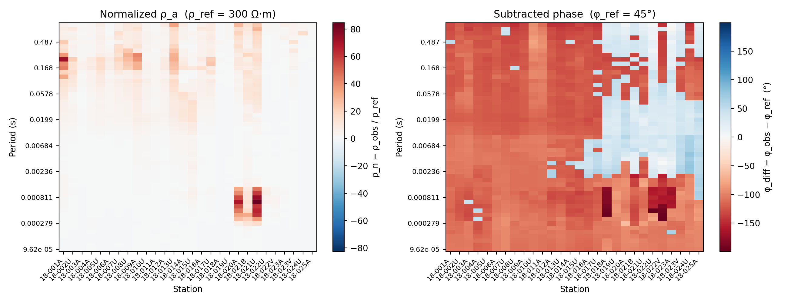
The left panel answers whether apparent resistivity is high or low
relative to the reference half-space; the longest-period row (top) is
where the near-field runaway already documented in
CSAMT Field-Zone Classification shows up here too, rho_n climbing past
10,000 at several stations – ten thousand times the reference
resistivity, not a real earth property. The right panel answers whether
phase is above or below the reference phase, and it is almost entirely
negative (red) across the section: observed phase runs well below the
45-degree far-field reference nearly everywhere, consistent with a
survey dominated by near- and transition-field rows rather than clean
plane-wave behaviour. Read both panels alongside the field-zone column
from normalize_response.
11.18.10. Near-Field Correction#
correct_near_field divides each impedance tensor row by a complex
near-field factor:
the equatorial horizontal-electric-dipole transfer-function ratio,
where \(k_1\) is the same complex earth wavenumber used above and
\(p\) is simply that wavenumber times the offset – a complex
version of the kr field-zone parameter, with \(|p| = kr\). The
factor tends toward 1 in the far field, where \(p\) is large
and the correction term vanishes. In the near field, where \(p\) is
small, dividing by \(3/p^3\) can make F very large, so the
correction can strongly change apparent resistivity.
>>> from pycsamt.emtools import correct_near_field
>>> corrected = correct_near_field(
...     sites,
...     source_offset=1000.0,
...     inplace=False,
... )
Use inplace=False while testing. If a correction changes a station by
orders of magnitude, treat that as a diagnostic result, not just a
processed output. It means the raw response was far from the plane-wave
assumption under the supplied offset – exactly what this survey’s
95-percent overprint rate and 69-percent near-field fraction already
predict.
11.18.11. Comparing Before And After#
You can compare source-effect diagnostics before and after correction without reaching into private helpers. For example, compare normalized response tables:
>>> from pycsamt.emtools import correct_near_field, ensure_sites, normalize_response
>>> raw = ensure_sites("data/CSAMT", recursive=False, strict=True)
>>> corrected = correct_near_field(raw, source_offset=1000.0, inplace=False)
>>> before = normalize_response(raw, rho_ref=1170.0, source_offset=1000.0)
>>> after = normalize_response(corrected, rho_ref=1170.0, source_offset=1000.0)
>>> joined = before.merge(
...     after,
...     on=["station", "freq_hz"],
...     suffixes=("_raw", "_corrected"),
... )
>>> joined["rho_n_ratio"] = joined["rho_n_corrected"] / joined["rho_n_raw"]
>>> joined[["station", "freq_hz", "zone_raw", "rho_n_raw", "rho_n_corrected", "rho_n_ratio"]].head()
  station    freq_hz    zone_raw  rho_n_raw  rho_n_corrected  rho_n_ratio
0  csa000  8196.7220         far   0.236752         0.236998     1.001039
1  csa000  4098.3610         far   0.646154         0.653463     1.011312
2  csa000  2049.1800  transition   1.581196         1.736024     1.097918
3  csa000  1023.5410  transition   3.632478         5.790342     1.594047
4  csa000   512.8206  transition   3.538460         1.617297     0.457062
The far row barely moves (ratio 1.001), exactly as expected
since F(p) -> 1 out there, while the two transition rows swing
by 60 percent and more in opposite directions – one pushed up, one
pulled down. This style keeps the comparison in public tables and is
easier to document than extracting impedance arrays directly.
11.18.12. Combining The Two Diagnostics#
The Yan/Fu beta flag and Wang/Lin field-zone label come from different physical arguments. Agreement between them is a strong warning that source geometry is controlling part of the response.
>>> from pycsamt.emtools import detect_source_overprint, normalize_response
>>> beta = detect_source_overprint(sites, source_offset=1000.0)
>>> zones = normalize_response(sites, rho_ref=1170.0, source_offset=1000.0)
>>> merged = beta.merge(
...     zones[["station", "freq_hz", "zone", "kr"]],
...     on=["station", "freq_hz"],
...     how="left",
... )
>>> merged.groupby("zone")["overprint_flag"].mean()
zone
far           0.2
near          1.0
transition    1.0
Name: overprint_flag, dtype: float64
>>> merged.groupby("zone")["beta_pct"].describe()
            count       mean        std  ...        50%        75%        max
zone                                     ...
far          10.0   1.386898   1.564839  ...   0.767703   2.125942   4.278410
near        118.0  49.917832   0.253333  ...  49.999891  49.999958  50.000025
transition   42.0  32.167391  13.282578  ...  34.197203  43.748063  47.611720

[3 rows x 8 columns]
Every near row and every transition row is overprint-flagged;
only 20 percent of far rows are. The two independent criteria agree
closely on this survey – both point to the same conclusion, that most
of this line’s usable band sits inside contaminated geometry at a 1 km
offset. If they disagreed instead, the right move would be to inspect
the assumed offset, reference resistivity, and frequency range before
trusting either one.
11.18.13. Choosing Offsets#
For real processing, offsets should come from survey geometry. A useful pattern is to build a station dictionary and pass it to every function – here a plausible taper reflecting a transmitter not perfectly centred on the line:
>>> from pycsamt.emtools import (
...     detect_source_overprint,
...     normalize_response,
...     source_overprint_table,
... )
>>> offset_by_station = {
...     "csa000": 950.0,
...     "csa050": 975.0,
...     "csa100": 1000.0,
...     "csa150": 1025.0,
...     "csa200": 1050.0,
...     "csa250": 1050.0,
...     "csa300": 1025.0,
...     "csa350": 1000.0,
...     "csa400": 975.0,
...     "csa450": 950.0,
... }
>>> detail2 = detect_source_overprint(sites, source_offset=offset_by_station)
>>> summary2 = source_overprint_table(sites, source_offset=offset_by_station)
>>> norm2 = normalize_response(sites, source_offset=offset_by_station)
>>> detail2["offset_m"].unique()
array([ 950.,  975., 1000., 1025., 1050.])
Keep the same offset dictionary across all source-effect diagnostics so the beta table, normalized-response table, field zones, and correction are comparable.
11.18.14. Suggested Review Sequence#
Use this sequence before applying a correction:
>>> detail = detect_source_overprint(sites, source_offset=1000.0)
>>> summary = source_overprint_table(sites, source_offset=1000.0, f_split=50.0)
>>> norm = normalize_response(sites, rho_ref=1170.0, source_offset=1000.0)
>>> detail["overprint_flag"].mean()
0.9529411764705882
>>> summary.sort_values("overprint_frac", ascending=False).head()
  station  n_freq  offset_m  ...  hf_slope  slope_delta  overprint_flag
4  csa200      17    1000.0  ... -0.339186    -0.632794            True
5  csa250      17    1000.0  ... -0.384489    -0.559169            True
0  csa000      17    1000.0  ... -0.893507    -0.055431            True
1  csa050      17    1000.0  ... -0.568374    -0.390639            True
2  csa100      17    1000.0  ... -0.679451    -0.263436            True

[5 rows x 11 columns]
>>> norm["zone"].value_counts(dropna=False)
zone
near          118
transition     42
far            10
Name: count, dtype: int64
Then plot:
>>> from pycsamt.emtools import plot_normalized_response, plot_overprint_section
>>> fig, ax = plt.subplots(figsize=(10, 5))
>>> _ = plot_overprint_section(sites, source_offset=1000.0, ax=ax)
>>> fig.tight_layout()
>>> fig.savefig("source_review_overprint_section_csamt.png", dpi=200)
>>> plt.close(fig)
>>> fig, axes = plt.subplots(1, 2, figsize=(13, 5))
>>> _ = plot_normalized_response(
...     sites,
...     rho_ref=1170.0,
...     source_offset=1000.0,
...     axes=axes,
... )
>>> fig.tight_layout()
>>> fig.savefig("source_review_normalized_response_csamt.png", dpi=200)
>>> plt.close(fig)
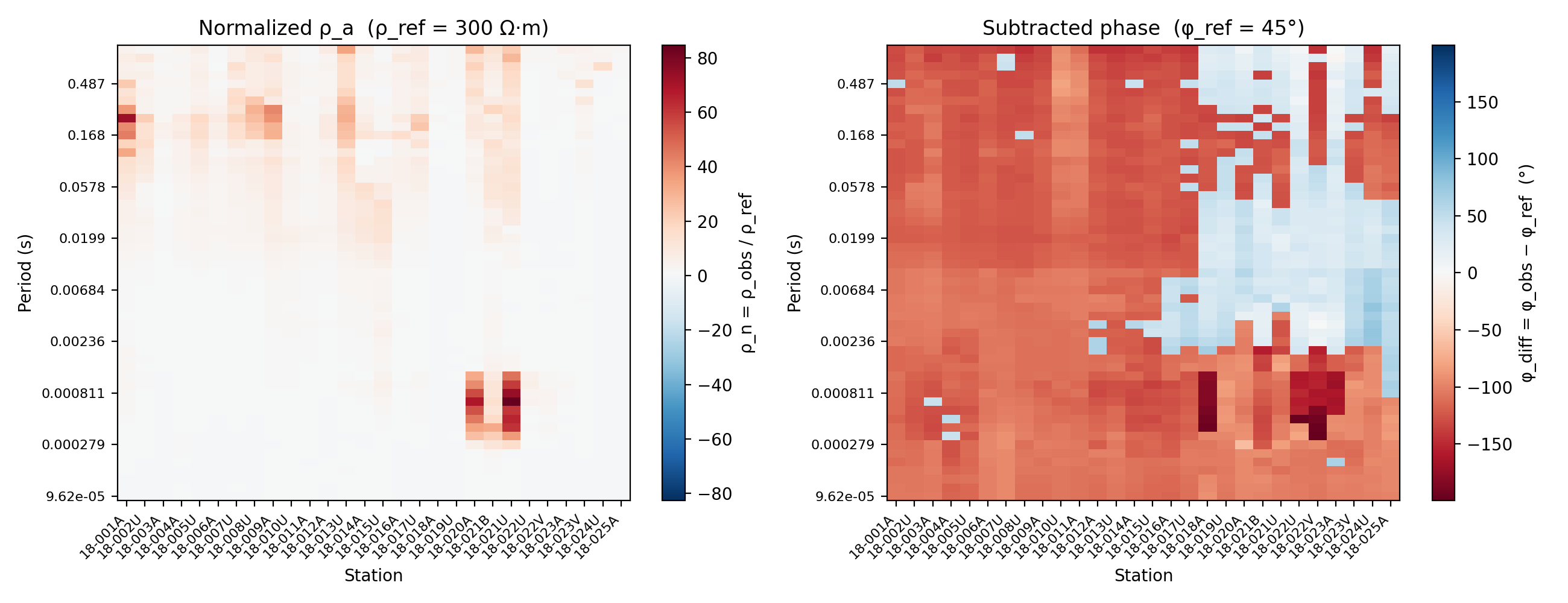
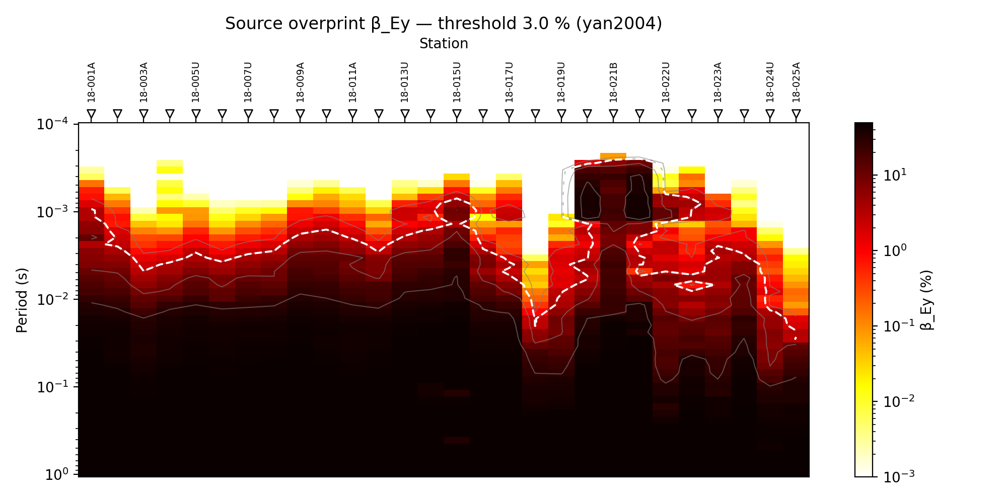
95 percent overprint-flagged, 69 percent near-field, and a normalized resistivity that climbs four orders of magnitude at long period all tell the same story from three different angles. Correct only after diagnostics like these show that correction is scientifically justified and after the offset geometry has been checked – on a survey this contaminated, correction is not optional polish, it is close to a prerequisite for any plane-wave interpretation at all.
11.18.15. Pitfalls#
Do not invent the source offset from the impedance. The offset is survey geometry and should come from field records or transmitter/receiver coordinates.
Do not interpret a representative scalar offset as a final result for a line with varying transmitter distance. A scalar is fine for examples or sensitivity tests; station-specific offsets are better for processing.
Do not treat near-field correction as harmless smoothing. It changes the impedance tensor and can alter apparent resistivity by large factors in near-field rows, as the 60-percent-plus swings in the before/after comparison above show directly.
Do not use the Da et al. slope columns without checking f_split. A
split outside the sampled frequency range produces undefined low- or
high-frequency slopes.
Do not expect normalize_response’s Wang and Lin field zones to land
on the same near/transition/far boundary as CSAMT Field-Zone Classification’s
Bostick-depth criterion at the same offset – they use different skin
depth scalings by design.
11.18.16. Worked Example#
The example uses the real Tongkeng CSAMT line with its actual 1 km transmitter offset. It demonstrates the pure beta formula, per-row overprint detection, station summaries, overprint pseudo-sections, normalized response, near-field correction, and comparison between the two independent source-effect diagnostics.
Open the rendered gallery page here: CSAMT source overprint and near-field effects (pycsamt.emtools.source_effects).