11.20. CSAMT Field-Zone Classification

pycsamt.emtools.fieldzone checks whether a controlled-source AMT measurement is far enough from the transmitter to behave like a plane-wave MT response. This matters because the usual apparent resistivity formula assumes far-field behavior. If the receiver is in the near field or transition field, apparent resistivity can be biased by the source geometry rather than only by subsurface structure.

This page is specific to controlled-source work. Natural-source AMT/MT does not have a transmitter-receiver offset, so running this module against it is a diagnostic exercise rather than evidence of genuine near-field bias. The examples below instead use pyCSAMT’s bundled real CSAMT survey, data/CSAMT – ten stations acquired over a grounded dipole transmitter for a groundwater-exploration study in the Tongkeng area, Hunan Province, China (Kouadio et al., 2020) [Kouadio2020]. The EDI files themselves do not carry the transmitter-receiver distance – that is field-notebook metadata, not part of the SEG EDI standard – so every example below still states its offset explicitly, but at least the transmitter genuinely exists.

In other words, the method is not a generic data-quality score. It asks a narrower physical question: at this frequency, resistivity level, and source-receiver distance, is the receiver many diffusion lengths away from the source, or is it still seeing the transmitter geometry directly?

Full callable signatures live in the API reference. This page focuses on the workflow, outputs, examples, and interpretation.

11.20.1. The Field-Zone Parameter

The core quantity is the dimensionless distance:

\[|k r| = {r \over \delta_B}.\]

where r is the source-receiver offset in metres and delta_B is the Bostick depth approximation:

\[\delta_B = 356 \sqrt{\rho_a \over f}.\]

Here \(f\) is frequency in hertz, \(\rho_a\) is apparent resistivity in ohm metres, and \(\delta_B\) is in metres. The constant 356 is the Bostick depth coefficient used by this module; it is the skin-depth scale divided by \(\sqrt{2}\). Thus \(|kr|\) is best read as source offset measured in Bostick-depth units.

The measured apparent resistivity is computed from the two off-diagonal impedance modes using the practical EDI convention used in pyCSAMT:

\[\rho_{xy} = 0.2 {|Z_{xy}|^2 \over f}, \qquad \rho_{yx} = 0.2 {|Z_{yx}|^2 \over f},\]

\[\rho_a = \sqrt{\rho_{xy}\rho_{yx}}.\]

The geometric mean keeps the field-zone diagnostic from depending on only one transverse mode. If one mode is noisy or locally distorted, the classification can still be affected, so treat the resulting zone as a geometry-and-response diagnostic rather than a replacement for ordinary impedance quality control.

Higher frequencies and larger offsets increase |k r| and push the measurement toward the far field. Larger apparent resistivity increases delta_B and can push the same offset back toward transition field or near field.

For fixed \(r\), the scaling is

\[|kr| \propto r\sqrt{f \over \rho_a}.\]

This compact relationship explains the main pattern in field-zone plots: short periods usually move downward toward far-field behavior, whereas long periods and high-resistivity intervals tend to move toward transition or near-field behavior.

11.20.2. Zone Rules

The default classification uses far_threshold = 3.0 and near_threshold = 0.3 on \(|kr|\):

\[\begin{split}\mathrm{zone}(|kr|) = \begin{cases} \text{far}, & |kr| \ge \tau_f, \\ \text{transition}, & \tau_n \le |kr| < \tau_f, \\ \text{near}, & |kr| < \tau_n, \end{cases}\end{split}\]

where \(\tau_f\) is far_threshold and \(\tau_n\) is near_threshold.

Interpret the zones as:

Zone	Practical meaning
far field	Plane-wave approximation is usually acceptable.
transition field	Source geometry may influence the response; inspect before inversion.
near field	Plane-wave apparent resistivity is not trustworthy without near-field correction or exclusion.

11.20.3. Offset Inputs

The field-zone functions need source_offset in metres. You can pass it in three ways:

Input	Meaning
source_offset=1000.0	Use one offset for every station.
source_offset={"csa000": 950.0, ...}	Use station-specific offsets.
source_offset=None	Try to read offset-like attributes from each station object.

When source_offset is a dictionary, missing stations are skipped unless the station object itself has an offset attribute. For real CSAMT, prefer station-specific offsets from survey geometry. Also note that these functions canonicalize station names to the EDI file stem (csa000, csa050, …) rather than the DATAID field recorded inside the file (S00, S01, …) – a dictionary keyed by DATAID would silently match nothing.

11.20.4. Classify Field Zones

Use classify_field_zones for the main per-station, per-frequency table.

>>> from pathlib import Path
>>> from pycsamt.emtools.fieldzone import classify_field_zones
>>> edi_dir = Path("data/CSAMT")
>>> zones = classify_field_zones(
...     edi_dir,
...     source_offset=1000.0,
...     far_threshold=3.0,
...     near_threshold=0.3,
...     recursive=False,
...     on_dup="replace",
...     strict=False,
...     verbose=0,
... )
>>> len(zones), zones["station"].unique().tolist()
(170, ['csa000', 'csa050', 'csa100', 'csa150', 'csa200', 'csa250', 'csa300', 'csa350', 'csa400', 'csa450'])
>>> zones.head()
  station    freq_hz  period_s  ...  delta_bostick_m         kr        zone
0  csa000  8196.7220  0.000122  ...        65.443971  15.280246         far
1  csa000  4098.3610  0.000244  ...       152.899372   6.540249         far
2  csa000  2049.1800  0.000488  ...       338.256213   2.956339  transition
3  csa000  1023.5410  0.000977  ...       725.423852   1.378504  transition
4  csa000   512.8206  0.001950  ...      1011.503356   0.988627  transition
[5 rows x 8 columns]
>>> zones.to_csv("tongkeng_field_zones.csv", index=False)
>>> zones["zone"].value_counts(normalize=True)
zone
near          0.635294
transition    0.241176
far           0.123529
Name: proportion, dtype: float64

The output columns are:

• station: station name.

• freq_hz and period_s: measured frequency and period.

• offset_m: source-receiver offset used for the calculation.

• rho_a_ohmm: determinant-style apparent resistivity.

• delta_bostick_m: Bostick depth approximation.

• kr: dimensionless |k r|.

• zone: far, transition, or near.

At a 1 km assumed offset – plausible for this survey’s transmitter layout – nearly two-thirds of this real ten-station CSAMT line’s station-period samples read as near field, and fewer than one in eight are safely far field. That is not a synthetic worst case: it is the genuine consequence of a Tongkeng-scale transmitter offset combined with the resistive, near-surface-dominated response typical of a groundwater-exploration target. The table is tidy: every row is one station-frequency sample. That shape is intentional because it lets you merge the result with QC, static-shift, skew, or inversion masks before deciding which periods to keep.

11.20.5. Single-Station Curve

Inspecting kr against period makes the classification easy to see.

>>> import matplotlib.pyplot as plt
>>> station = "csa000"
>>> one = zones.loc[zones["station"] == station].sort_values("period_s")
>>> fig, ax = plt.subplots(figsize=(7, 4.5))
>>> _ = ax.axhspan(3.0, 1e6, color="tab:green", alpha=0.08)
>>> _ = ax.axhspan(0.3, 3.0, color="tab:orange", alpha=0.10)
>>> _ = ax.axhspan(1e-6, 0.3, color="tab:red", alpha=0.08)
>>> _ = ax.loglog(one["period_s"], one["kr"], "o-", color="0.2")
>>> _ = ax.axhline(3.0, color="0.4", linestyle="--")
>>> _ = ax.axhline(0.3, color="0.4", linestyle="--")
>>> _ = ax.set_xlabel("Period (s)")
>>> _ = ax.set_ylabel("|k r|")
>>> _ = ax.set_title(f"{station} field-zone parameter")
>>> fig.tight_layout()

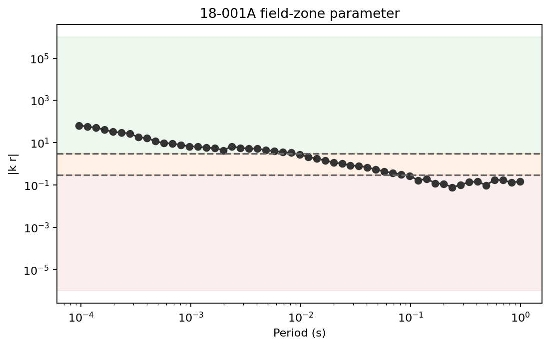
The shaded regions show the far, transition, and near zones. csa000 (the profile’s 0 m station) only clears the far-field line at its two highest measured frequencies; everything below roughly 2 Hz has already fallen into the near field at this offset – long periods move toward smaller kr because Bostick depth increases as frequency decreases, and it does not take a very long period to outrun a 1 km transmitter offset here.

11.20.6. Near-Field Factor

near_field_factor computes a continuous correction factor for the equatorial horizontal electric dipole approximation:

\[F(p) = 1 - {3 \over p^2} + {3 \over p^3}\]

where p = k r is complex. The returned nf_factor is abs(F). When it is close to 1, the response is far-field-like. Large departures indicate near-field bias. Apparent resistivity bias scales approximately with abs(F)^2.

The complex wavenumber used for this factor is

\[k = {1+i \over \sqrt{2}} \sqrt{\omega\mu_0 \over \rho_a}, \qquad \omega = 2\pi f,\]

so

\[p = k r.\]

The classification parameter uses only the magnitude scale \(|kr|\), while nf_factor keeps the phase of the diffusive wavenumber. That is why the two outputs are complementary: zone is easy to threshold and map; nf_factor shows how quickly the near-field expression departs from the far-field limit.

>>> from pycsamt.emtools.fieldzone import near_field_factor
>>> survey = "data/CSAMT"
>>> offset_m = 1000.0
>>> factors = near_field_factor(survey, offset_m)
>>> merged = zones.merge(
...     factors[["station", "freq_hz", "nf_factor"]],
...     on=["station", "freq_hz"],
...     how="inner",
... )
>>> merged.groupby("zone")["nf_factor"].agg(["count", "mean", "median", "max"])
            count          mean        median           max
zone
far            21  9.882218e-01  9.899938e-01  9.994810e-01
near          108  9.078250e+09  1.848531e+06  2.087716e+11
transition     41  7.138050e+00  9.543661e-01  5.656376e+01

This cross-check is useful because zone is threshold-based, while nf_factor is continuous. In a good classification, far-zone samples should cluster near nf_factor = 1 (they do: mean 0.988), and near-zone samples should show larger departures. On real data they show much larger departures than a synthetic example would suggest: the near-zone mean is dominated by the survey’s lowest measured frequency (0.125 Hz), where apparent resistivity climbs past ten million ohm-metres at several stations (up to 16.7 million at csa350) – the textbook signature of geometric near-field runaway, not a resolved deep layer.

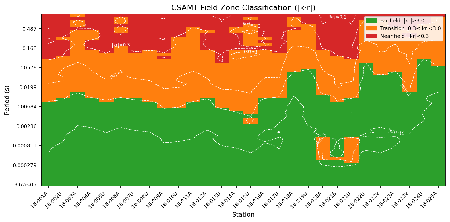
11.20.7. Plot Field Zones

plot_field_zones maps zone labels onto station x period space and can overlay |k r| contours.

The plotted image is a matrix

\[Z_{ij} = \mathrm{zone}\left(|kr|_{ij}\right),\]

where \(i\) indexes period or frequency and \(j\) indexes station. Dashed contours are drawn from the continuous \(|kr|_{ij}\) grid, so the colors show the thresholded decision and the contours show how close each area is to a boundary.

>>> from pycsamt.emtools.fieldzone import plot_field_zones
>>> fig, ax = plt.subplots(figsize=(10, 5))
>>> _ = plot_field_zones(
...     "data/CSAMT",
...     source_offset=1000.0,
...     far_threshold=3.0,
...     near_threshold=0.3,
...     contour_kr=True,
...     kr_levels=(0.1, 0.3, 1.0, 3.0, 10.0),
...     sort_by="name",
...     period_axis=True,
...     ax=ax,
... )
>>> ax.get_title()
'CSAMT Field Zone Classification (|k·r|)'

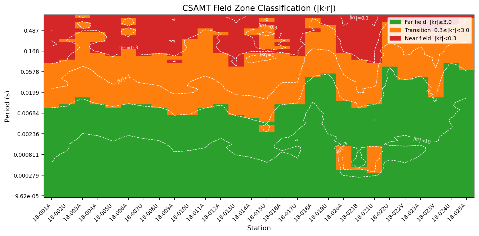
Use this as the main survey view. The near field sets in early (at high frequency, short period) across nearly the whole profile, with a slightly more resistive patch around csa150-csa200 pushing the far/transition boundary out to a longer period than its neighbours. A broad red or orange band at long periods means those periods should be excluded, corrected, or treated with caution before plane-wave inversion – here, that is most of the sounding.

11.20.8. Station-Specific Offsets

Real CSAMT geometry often varies by station. Pass a dictionary when each station has its own source-receiver distance.

>>> offsets_m = {
...     "csa000": 950.0,
...     "csa100": 1000.0,
...     "csa200": 1050.0,
... }
>>> zones_subset = classify_field_zones(
...     "data/CSAMT",
...     source_offset=offsets_m,
...     recursive=False,
...     verbose=1,
... )
>>> zones_subset["station"].unique()
array(['csa000', 'csa100', 'csa200'], dtype=object)
>>> len(zones_subset)
51

Only stations with offsets are classified – the other seven stations in this survey are silently dropped here, which is why len is 51 (3 stations times 17 frequencies) rather than 170. With verbose=1, missing offsets produce warnings from the classifier. In production workflows, build this dictionary from the transmitter and receiver coordinates, keyed by the canonicalized station name described above.

11.20.9. Offset Sensitivity

If the source offset is uncertain, run a sensitivity sweep. The same observed impedances can move between far and near zones solely because the assumed offset changes.

For an assumed offset \(r_m\), the zone fraction is

\[P_z(r_m) = {1 \over N} \sum_{s,f} \mathbf{1}\left[ \mathrm{zone}_{s,f}(r_m) = z \right],\]

where \(N\) is the number of classified station-frequency samples. This is a simple summary, but it is very effective at exposing whether a processing conclusion depends on an assumed transmitter distance.

>>> import pandas as pd
>>> offsets = [500.0, 1000.0, 2000.0, 8000.0]
>>> rows = []
>>> for offset in offsets:
...     z = classify_field_zones(survey, source_offset=offset)
...     fractions = z["zone"].value_counts(normalize=True)
...     rows.append(
...         {
...             "offset_m": offset,
...             "far": fractions.get("far", 0.0),
...             "transition": fractions.get("transition", 0.0),
...             "near": fractions.get("near", 0.0),
...         }
...     )
...
>>> sensitivity = pd.DataFrame(rows)
>>> sensitivity
   offset_m       far  transition      near
0     500.0  0.058824    0.247059  0.694118
1    1000.0  0.123529    0.241176  0.635294
2    2000.0  0.211765    0.211765  0.576471
3    8000.0  0.358824    0.217647  0.423529

Report this table when offset is assumed rather than measured. It makes the geometry dependence visible instead of hiding it inside one plot. Notice how slowly the near-field fraction falls here – even at an 8 km offset, eight times the primary assumption, 42 percent of this survey is still near field. That resistant tail is itself informative: a shallow, highly resistive target keeps pushing Bostick depth (and therefore |kr|) down no matter how far the assumed transmitter moves, which is exactly the behaviour a groundwater-exploration CSAMT line over near-surface resistive structure should show.

11.20.10. Comparing Offsets Side By Side

The plotting function accepts ax so several assumed offsets can be compared in one figure.

>>> fig, (ax_near, ax_far) = plt.subplots(1, 2, figsize=(13, 5), sharey=True)
>>> _ = plot_field_zones(survey, source_offset=500.0, ax=ax_near)
>>> _ = ax_near.set_title("Offset = 500 m")
>>> _ = plot_field_zones(survey, source_offset=8000.0, ax=ax_far)
>>> _ = ax_far.set_title("Offset = 8000 m")
>>> fig.tight_layout()

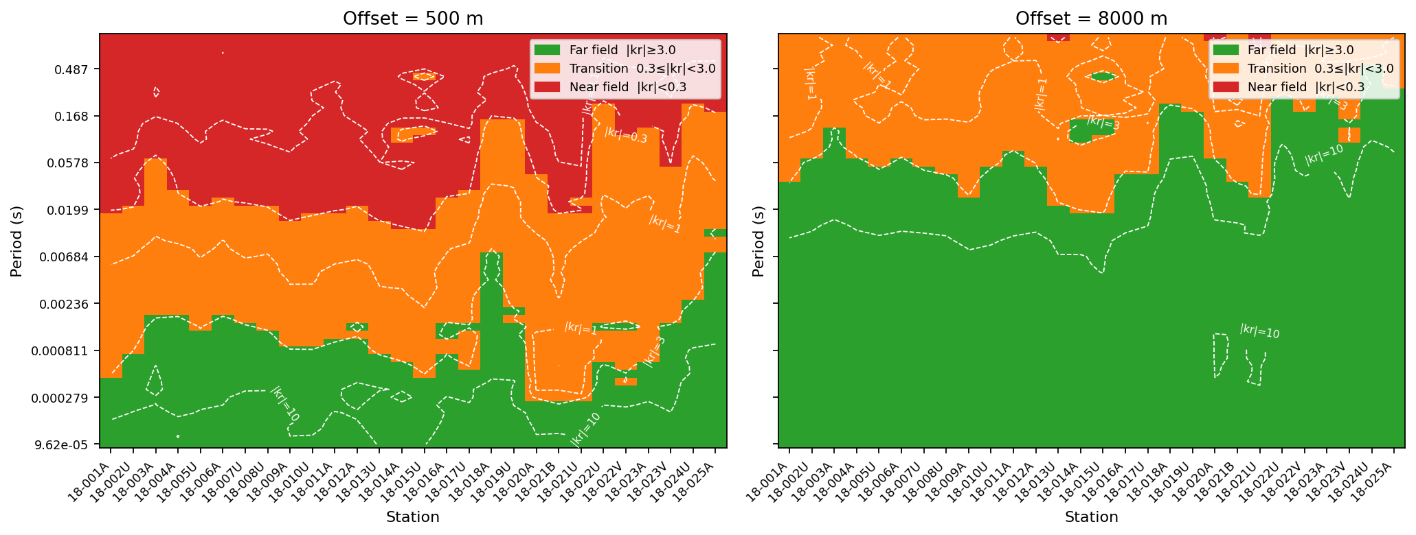
This comparison is especially useful for design studies: if the target period band is near or transition at the planned offset, move the source, change the frequency band, or plan controlled-source corrections. Here, even the generously far 8 km panel keeps a substantial red near-field band at long period – widening the offset helps, but it does not rescue this survey’s longest periods.

11.20.11. Illustrative Near-Field Correction

The near-field factor can show how strongly a sounding might be biased. The example below divides apparent resistivity by nf_factor ** 2 as an illustrative correction. Use the appropriate controlled-source convention and survey geometry before applying this in production.

The illustrative curve is

\[\rho_a^\mathrm{illustrative} = {\rho_a^\mathrm{measured} \over |F(p)|^2}.\]

This follows the module’s equatorial HED approximation, where the field amplitude bias enters apparent resistivity as a squared factor. It is a diagnostic visualization, not a universal correction recipe for every CSAMT transmitter layout.

>>> one_merged = merged.loc[merged["station"] == station].sort_values("period_s")
>>> corrected = one_merged["rho_a_ohmm"] / (one_merged["nf_factor"] ** 2)
>>> fig, ax = plt.subplots(figsize=(7, 4.5))
>>> _ = ax.loglog(one_merged["period_s"], one_merged["rho_a_ohmm"], "o-", label="measured")
>>> _ = ax.loglog(one_merged["period_s"], corrected, "s--", label="illustrative / |F|^2")
>>> _ = ax.set_xlabel("Period (s)")
>>> _ = ax.set_ylabel("Apparent resistivity (ohm.m)")
>>> _ = ax.legend()
>>> fig.tight_layout()

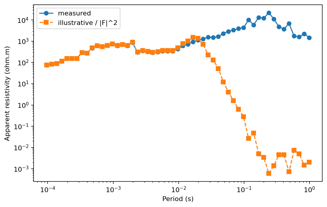
Where nf_factor is near 1, the curves overlap – true here only at the shortest two or three periods. Past that, the curves do not just separate: the illustrative correction collapses to physically meaningless values, down to about \(1.7\times10^{-15}\ \Omega\cdot\mathrm{m}\) at the longest (8 s) period, because csa000’s own nf_factor reaches \(\sim6.7\times10^{10}\) there and the correction divides by its square. That collapse is itself the honest result, not a plotting artefact: dividing by an astronomically large factor cannot recover a real earth resistivity, and a station this deep in the near field needs a genuine controlled-source inversion or exclusion, not a scalar correction. Treat any station-period cell where the illustrative curve has fallen off a cliff like this one as a demonstration of why the correction is illustrative, not as a usable corrected value.

11.20.12. Reading The Results

Use this interpretation order:

• Confirm the source offset is real and in metres.

• Inspect kr and zone before using long-period CSAMT data in a plane-wave inversion.

• Treat transition samples as conditional, not automatically safe.

• Use near_field_factor to quantify how severe the departure from far-field behavior may be.

• Run offset sensitivity when the source geometry is assumed or uncertain.

• Prefer station-specific offsets when transmitter-receiver geometry is available.

11.20.13. Common Failure Modes

Empty output

No valid impedance tensors were loaded, or no source offset could be resolved for any station.

Natural-source data without offsets

AMT/MT data do not carry a transmitter offset. You can run sensitivity examples with assumed offsets, but do not present those numbers as measured survey geometry, and remember that the whole exercise is illustrative rather than diagnostic without a real transmitter.

Wrong offset units

Offsets must be metres. Passing kilometres without conversion will severely misclassify the field zone.

One offset for a whole survey

This is acceptable for illustration or a constant-offset acquisition, but station-specific geometry is safer for real CSAMT.

Far-zone label at noisy frequencies

Field-zone classification only checks source geometry and apparent resistivity. It does not replace quality control.

Station-name mismatch in offset dictionaries

source_offset dictionaries are matched against the canonicalized station name (the EDI file stem), not necessarily the DATAID recorded inside the file. A dictionary keyed by the wrong name silently classifies zero stations instead of raising an error.

11.20.14. Saving A Reproducible Bundle

For reports, save the classification table, near-field factor table, offset-sensitivity summary, and field-zone pseudo-section.

>>> from pathlib import Path
>>> out = Path("outputs/fieldzone_tongkeng")
>>> out.mkdir(parents=True, exist_ok=True)
>>> zones.to_csv(out / "field_zones.csv", index=False)
>>> factors.to_csv(out / "near_field_factor.csv", index=False)
>>> sensitivity.to_csv(out / "offset_sensitivity.csv", index=False)
>>> fig, ax = plt.subplots(figsize=(10, 5))
>>> _ = plot_field_zones(survey, offset_m, ax=ax)
>>> fig.tight_layout()
>>> fig.savefig(out / "field_zone_pseudosection.png", dpi=200)

11.20.15. Worked Example

The gallery example uses the real ten-station Tongkeng CSAMT survey (data/CSAMT) with an assumed but plausible 1 km transmitter offset. It demonstrates the |k r| relationship, one-station curves, near-field factor cross-checks, pseudo-sections, offset sensitivity, and an illustrative near-field correction, all against a survey where a controlled source genuinely exists.

Open the rendered example here: CSAMT field-zone classification (pycsamt.emtools.fieldzone).