18.3. Inspect and QC a Survey#

This tutorial shows how to perform a first-pass quality-control review of an EDI survey before correction, recomputation, modelling, or inversion. The goal is not to decide the final geophysical interpretation. The goal is to answer a more practical question:

Which stations and frequency bands are reliable enough to use first, and which ones need manual review?

The workflow follows the style used throughout pyCSAMT v2:

read the survey once
inspect the station inventory
build compact station-level QC tables
compute confidence scores
identify stations and frequency bands that need attention
save review tables and diagnostic plots
use CLI commands for quick checks where they are available

18.3.1. What You Will Learn#

After this tutorial you should be able to:

load one EDI file, one survey directory, or a recursive survey tree
inspect station names, frequency coverage, and missing transfer functions
create a station-level quality-control table with pycsamt.emtools.qc.build_qc_table()
generate simple flags with pycsamt.emtools.qc.qc_flags()
compute station and frequency confidence tables
export QC results for a field notebook, spreadsheet, or processing report
choose which stations to keep, review, recompute, or remove from the first inversion trial

18.3.2. Input Assumptions#

The examples below use the bundled WILLY L18PLT line:

data/AMT/WILLY_DATA/L18PLT

Replace that path with your own EDI directory when you repeat the workflow on student, field, or project data. The path can be:

a single .edi file
a directory containing EDI files
a survey directory with line subdirectories

For example:

my_project/
  edis/
    line_01/
      S001.edi
      S002.edi
    line_02/
      S101.edi
      S102.edi

When a directory contains several lines, use recursive=True so pyCSAMT discovers EDI files below the top-level folder.

18.3.3. Load the Survey#

Start by reading the EDI survey through the public API. strict=False is useful during the first inspection because it allows the reader to continue past recoverable metadata issues.

>>> from pycsamt.api import read_edis
>>> edi_dir = "data/AMT/WILLY_DATA/L18PLT"
>>> survey = read_edis(
...     edi_dir,
...     recursive=False,
...     strict=False,
...     progress=False,
... )
>>> sites = survey.collection
>>> print(survey.summary())
APIFrame: edi_survey_summary
kind: edi.summary
shape: 28 rows x 6 columns
columns: station, path, n_freq, tipper, spectra, ts
numeric: 1 columns
missing: 0.0%
source: data/AMT/WILLY_DATA/L18PLT

survey is the public survey object returned by the API. sites is the site collection used by most station editing, computation, and QC helpers. The summary confirms all 28 stations were loaded, with no missing values and a single numeric column (n_freq) – a first, coarse signal that loading itself did not silently drop or corrupt anything.

If you only need a pandas-friendly station inventory, inspect the survey summary table:

>>> inventory = survey.df.to_pandas(copy=True)
>>> print(inventory.columns.tolist())
['station', 'path', 'n_freq', 'tipper', 'spectra', 'ts']
>>> other_cols = ["station", "n_freq", "tipper", "spectra", "ts"]
>>> print(inventory[other_cols].head(3).to_string(index=False))
   station  n_freq  tipper  spectra    ts
23-18-001A      53   False    False False
23-18-002U      53   False    False False
23-18-003A      53   False    False False

inventory["path"] is omitted from the printed table above because it resolves to an absolute filesystem path, which differs by machine; inspect it directly (inventory["path"].iloc[0]) to confirm each row points at the EDI file you expect.

The 23- prefix on every station value here is not a typo: the raw EDI header’s own DATAID field is "23-18-001A" (grep DATAID 18-001A.edi), encoding the 2023 acquisition year ahead of the line/station code, and survey.df reports that field as-is. The QC and confidence tables built below instead key on the file-stem-derived 18-001A form, so the two identifiers must be matched by their common 18-NNNx suffix, not assumed identical – a real, worth-noticing detail rather than a display quirk. At this stage, also check that the number of stations is what you expected, that station names are not duplicated unintentionally, and that the frequency count (53 here, for every row) is consistent across the line – a ragged n_freq column would mean some stations lost frequencies during acquisition or parsing.

18.3.4. Create an Output Folder#

QC usually produces several small tables and plots. Put them in one folder so the review is reproducible.

>>> from pathlib import Path
>>> qc_dir = Path("qc_review")
>>> qc_dir.mkdir(exist_ok=True)

18.3.5. Build the Station QC Table#

The first compact table is produced by pycsamt.emtools.qc.build_qc_table(). It summarizes the usable impedance rows per station and, when possible, adds simple phase-tensor skew diagnostics.

>>> from pycsamt.emtools.qc import build_qc_table
>>> qc = build_qc_table(
...     sites,
...     include_skew=True,
...     recursive=False,
...     api=True,
... )
>>> qc_df = qc.to_pandas(copy=True)
>>> cols = ["station", "n_freq", "frac_ok", "snr_med", "skew_med", "pmin", "pmax"]
>>> print(qc_df[cols].head(5).to_string(index=False))
station  n_freq  frac_ok   snr_med  skew_med     pmin     pmax
18-001A      53      1.0 17.658396  4.809977 0.000096 0.992063
18-002U      53      1.0 16.687366  6.596544 0.000096 0.992063
18-003A      53      1.0 12.031672 11.018588 0.000096 0.992063
18-004A      53      1.0 10.430580 14.509282 0.000096 0.992063
18-005U      53      1.0 14.360341  9.171151 0.000096 0.992063

The important teaching point is that complete coverage does not mean the data are automatically ready for inversion. This line has frac_ok = 1.0 at every station shown, but skew_med already varies by a factor of three across just these five stations (4.8 to 14.5 degrees), which is enough on its own to justify the dimensionality review in Dimensionality, Distortion, And The Phase Tensor before trusting a 1-D/2-D interpretation anywhere on this line.

The most useful columns are:

station: Station name inferred from the EDI object.
n_freq: Number of frequency rows available at the station.
n_ok: Number of rows where the impedance tensor is finite enough for QC.
frac_ok: Fraction of usable impedance rows, from 0 to 1.
n_tip and n_tip_ok: Number of tipper rows and usable tipper rows when tipper data are present.
snr_med: Median signal-to-noise proxy derived from impedance values and impedance errors when error tensors are available.
pmin and pmax: Shortest and longest periods represented by the station.
skew_med and skew_iqr: Median absolute phase-tensor skew and its interquartile spread. These columns are only added when include_skew=True.

Export the table:

>>> qc_df.to_csv(qc_dir / "station_qc.csv", index=False)

18.3.6. Sort Stations by Review Priority#

A practical first review is to sort stations by coverage and signal quality.

>>> review_order = qc_df.sort_values(
...     by=["frac_ok", "snr_med"],
...     ascending=[True, True],
... )
>>> print(review_order[cols].head(15).to_string(index=False))
station  n_freq  frac_ok   snr_med  skew_med     pmin     pmax
18-022U      53      1.0  8.557456 49.751057 0.000096 0.992063
18-024U      53      1.0  8.987776 11.482211 0.000096 0.992063
18-021B      53      1.0  9.339868 47.235914 0.000096 0.992063
18-023A      53      1.0  9.854384 54.529465 0.000096 0.992063
18-004A      53      1.0 10.430580 14.509282 0.000096 0.992063
18-022V      53      1.0 11.268011 36.986632 0.000096 0.992063
18-025A      53      1.0 11.770850 24.634843 0.000096 0.992063
18-013U      53      1.0 11.944265 12.025504 0.000096 0.992063
18-003A      53      1.0 12.031672 11.018588 0.000096 0.992063
18-023V      53      1.0 12.137127 14.611436 0.000096 0.992063
18-011A      53      1.0 12.575896  9.310687 0.000096 0.992063
18-012A      53      1.0 12.873938  9.052529 0.000096 0.992063
18-006A      53      1.0 13.272516 12.375357 0.000096 0.992063
18-015U      53      1.0 13.456819 14.242493 0.000096 0.992063
18-010U      53      1.0 13.677553  9.242375 0.000096 0.992063

Stations near the top of this sorted table should be checked before automated static-shift correction, dimensionality analysis, or inversion preparation. In this line, the sort mostly separates stations by signal-quality proxy because the frequency coverage is complete at every station – but note that sorting by snr_med alone does not track skew_med: 18-022U (lowest SNR) has skew_med=49.8, comparable to 18-023A further down the list (skew_med=54.5, the highest of these 15), while 18-024U sits second from the bottom on SNR yet has one of the lowest skew values shown (11.5). Low SNR and high skew are different failure modes – a station can have either, both, or neither – so a single sort column is a starting point for review, not a complete ranking.

18.3.7. Create Simple QC Flags#

Use pycsamt.emtools.qc.qc_flags() to attach simple rule-based labels. The thresholds below are intentionally conservative for a first review. Adjust them for local data quality, acquisition style, and survey objectives.

>>> from pycsamt.emtools.qc import qc_flags
>>> flagged = qc_flags(
...     sites,
...     min_frac_ok=0.75,
...     min_snr_med=3.0,
...     max_skew_med=6.0,
...     recursive=False,
... )
>>> flagged.to_csv(qc_dir / "station_qc_flags.csv", index=False)
>>> print(flagged[["station", "frac_ok", "snr_med", "flags"]].head(5).to_string(index=False))
station  frac_ok   snr_med     flags
18-001A      1.0 17.658396
18-002U      1.0 16.687366 high_skew
18-003A      1.0 12.031672 high_skew
18-004A      1.0 10.430580 high_skew
18-005U      1.0 14.360341 high_skew
>>> print(flagged["flags"].value_counts().to_string())
flags
high_skew    27
              1

With this conservative max_skew_med=6.0 threshold, 27 of the 28 stations receive high_skew. That is not an instruction to remove the whole line. It is a clear sign that the next review should include phase-tensor, strike, geology, and inversion residual diagnostics before trusting a simple 1-D/2-D model anywhere on this profile. The sole exception, 18-001A (skew_med=4.8, visible in the table above), is worth remembering as a reference point precisely because it is the outlier: if a later diagnostic disagrees with it specifically, that disagreement is more informative than one more station agreeing with the crowd.

Typical flags are:

low_coverage: Too few usable impedance rows. This can indicate incomplete spectra, parsing problems, bad frequency windows, or severe masking.
low_snr: The median signal-to-noise proxy is below the selected threshold.
high_skew: Phase-tensor skew is high enough to deserve dimensionality review.

A flag is not a deletion instruction. It is a review instruction. In field datasets, low confidence can be caused by a real local conductor, poor electrode contact, cultural noise, incorrect coordinate metadata, a rotation mismatch, or format conversion from another software package.

18.3.8. Compute Station Confidence#

The QC table is compact. The confidence table is more diagnostic. It combines several indicators into a normalized confidence score between 0 and 1.

>>> from pycsamt.emtools.qc import station_confidence_table
>>> station_ci = station_confidence_table(
...     sites,
...     method="composite",
...     relerr_threshold=0.20,
...     offdiag_tolerance_log10=0.35,
...     diagonal_leakage_max=0.35,
...     phase_jump_tolerance_deg=90.0,
...     spatial_tolerance_log10=0.60,
...     spacing_m=200.0,
...     recursive=False,
...     api=True,
... )
>>> station_ci_df = station_ci.to_pandas(copy=True)
>>> station_ci_df.to_csv(qc_dir / "station_confidence.csv", index=False)
>>> ci_cols = ["station", "distance_m", "confidence", "confidence_err",
...            "coverage", "uncertainty", "offdiag", "diagonal", "phase", "spatial"]
>>> print(station_ci_df[ci_cols].head(3).to_string(index=False))
station  distance_m  confidence  confidence_err  coverage  uncertainty  offdiag  diagonal    phase  spatial
18-001A         0.0    0.709038        0.342984       1.0     0.716714 0.462176  0.000000 0.975510 0.488179
18-002U       200.0    0.774634        0.265434       1.0     0.561796 0.551179  0.328771 0.976991 0.990216
18-003A       400.0    0.713303        0.247746       1.0     0.551732 0.452082  0.387056 0.971592 0.492792

The confidence score is lower than the coverage score because it includes tensor consistency, diagonal leakage, phase continuity, and spatial coherence. 18-001A makes the point concretely: coverage=1.0 (every impedance row is usable) but confidence=0.709, dragged down mainly by diagonal=0.0 – the diagonal-leakage check fails outright at this station even though the earlier QC table showed it as the one station without a high_skew flag. Coverage, skew, and diagonal leakage are measuring different things, and a station can pass one check while failing another.

Important confidence columns include:

confidence: Composite score. Values close to 1 are usually safer for first-pass modelling. Values near 0 need review.
confidence_err: Uncertainty proxy for the confidence score.
coverage: Fraction of finite impedance rows.
uncertainty: Score derived from impedance error tensors when available.
offdiag: Consistency score between the two off-diagonal impedance components.
diagonal: Score based on diagonal leakage relative to the off-diagonal components.
phase: Score based on abrupt phase jumps.
spatial: Neighbor-coherence score along the station profile.

18.3.9. Review Low-Confidence Stations#

For first-pass work, a common pattern is to review stations below 0.6 and start inversion tests with stations above 0.8. These are practical defaults, not universal geophysical laws.

>>> low_ci = station_ci_df[station_ci_df["confidence"] < 0.60]
>>> high_ci = station_ci_df[station_ci_df["confidence"] >= 0.80]
>>> print("stations to review")
stations to review
>>> print(low_ci[["station", "confidence", "coverage", "phase", "spatial"]].to_string(index=False))
station  confidence  coverage    phase  spatial
18-017U    0.595479       1.0 0.969783 0.038160
18-018A    0.578410       1.0 0.957546 0.000000
18-021U    0.594344       1.0 0.938165 0.233576
18-021B    0.574114       1.0 0.937891 0.232771
18-022U    0.544020       1.0 0.941638 0.000000
>>> print("stations suitable for first trials")
stations suitable for first trials
>>> print(high_ci[["station", "confidence", "coverage"]].to_string(index=False))
station  confidence  coverage
18-007U    0.811922       1.0
>>> low_ci.to_csv(qc_dir / "stations_to_review.csv", index=False)

Five stations fall below 0.60 and exactly one, 18-007U, clears the 0.80 bar – 22 of the 28 stations sit in the wide middle ground between those thresholds, which is a routine outcome for a real field line, not a survey failure. 18-021U and 18-021B sit next to each other in station order and both land in the review group with nearly identical spatial scores (0.234 and 0.233); their spatial score is well above the 18-018A/18-022U pair, whose spatial=0.0 means each disagrees sharply with its immediate neighbours rather than sharing a trend with them. That distinction matters for the next step: a shared low score across adjacent stations points toward a regional cause (cultural noise, a real geologic contact, a survey-wide processing choice), while an isolated spatial=0.0 station points toward something local to that one station – acquisition metadata, electrode layout, orientation, or file conversion history.

18.3.10. Inspect Frequency-Level Confidence#

Station averages can hide narrow-band problems. Use pycsamt.emtools.qc.frequency_confidence_table() to inspect every station-frequency sample.

>>> from pycsamt.emtools.qc import frequency_confidence_table
>>> freq_ci = frequency_confidence_table(
...     sites,
...     method="composite",
...     ci_hi=0.95,
...     ci_lo=0.50,
...     recursive=False,
...     api=True,
... )
>>> freq_ci_df = freq_ci.to_pandas(copy=True)
>>> freq_ci_df.to_csv(qc_dir / "frequency_confidence.csv", index=False)
>>> weak_freq = freq_ci_df[freq_ci_df["confidence"] < 0.50]
>>> len(weak_freq), len(freq_ci_df)
(68, 1484)
>>> weak_cols = ["station", "frequency_hz", "period_s", "confidence", "flags"]
>>> print(weak_freq[weak_cols].head(6).to_string(index=False))
station  frequency_hz  period_s  confidence                                                               flags
18-003A      2997.000  0.000334    0.480450                  reject,high_error,offdiag_mismatch,spatial_outlier
18-003A         1.438  0.695410    0.485396 reject,high_error,offdiag_mismatch,diagonal_leakage,spatial_outlier
18-003A         1.008  0.992063    0.477361 reject,high_error,offdiag_mismatch,diagonal_leakage,spatial_outlier
18-004A      4277.000  0.000234    0.490229 reject,high_error,offdiag_mismatch,diagonal_leakage,spatial_outlier
18-004A      3580.000  0.000279    0.456718 reject,high_error,offdiag_mismatch,diagonal_leakage,spatial_outlier
18-004A      2997.000  0.000334    0.496109 reject,high_error,offdiag_mismatch,diagonal_leakage,spatial_outlier

The line has 68 station-frequency rows below 0.50 confidence out of 1,484 total (28 stations x 53 frequencies) – under 5% of the whole survey, concentrated rather than spread evenly:

>>> weak_freq["station"].nunique()
19
>>> print(weak_freq["station"].value_counts().head(5).to_string())
station
18-022U    12
18-023A    12
18-006A     6
18-021B     5
18-013U     5

Nineteen of the 28 stations contribute at least one weak frequency row, but the counts are uneven, and comparing this list against the station-level confidence table above is the useful step. 18-022U was already flagged there (confidence=0.544), so 12 weak frequency rows are consistent with its low station average. 18-023A was not flagged – its station-level confidence is comfortably above the 0.60 review threshold – yet it ties 18-022U for the most weak frequency rows on the whole line. That is exactly the failure mode this section opened with: a station average can hide a narrow-band problem. 18-023A deserves a frequency-level look even though the station-level table alone would not have flagged it. The flags column also shows why each row is weak (high_error, offdiag_mismatch, diagonal_leakage, spatial_outlier): a row flagged only spatial_outlier calls for a different response (compare with neighbours, check coordinates) than one also flagged diagonal_leakage (revisit component orientation or genuine 3-D structure at that frequency).

The frequency table is useful when you want to:

mask a narrow noisy band rather than remove a whole station
compare confidence between short-period and long-period data
find stations with repeated phase jumps
identify frequencies that may be affected by source-field instability, dead-band behavior, or cultural noise

18.3.11. Create a Confidence Profile Plot#

A line plot helps decide whether poor confidence is isolated, clustered, or profile-wide.

>>> import matplotlib.pyplot as plt
>>> from pycsamt.emtools.qc import plot_confidence_profile
>>> ax = plot_confidence_profile(
...     sites,
...     method="composite",
...     ci_hi=0.95,
...     ci_lo=0.50,
...     station_labels=True,
...     spacing_m=200.0,
...     recursive=False,
... )
>>> ax.figure.savefig(
...     qc_dir / "station_confidence_profile.png",
...     dpi=200,
...     bbox_inches="tight",
... )
>>> plt.close(ax.figure)

The tutorial figures are generated by docs/scripts/generate_tutorial_inspect_qc.py from the same code path. The first figure compares the station-level SNR proxy with the composite confidence score:

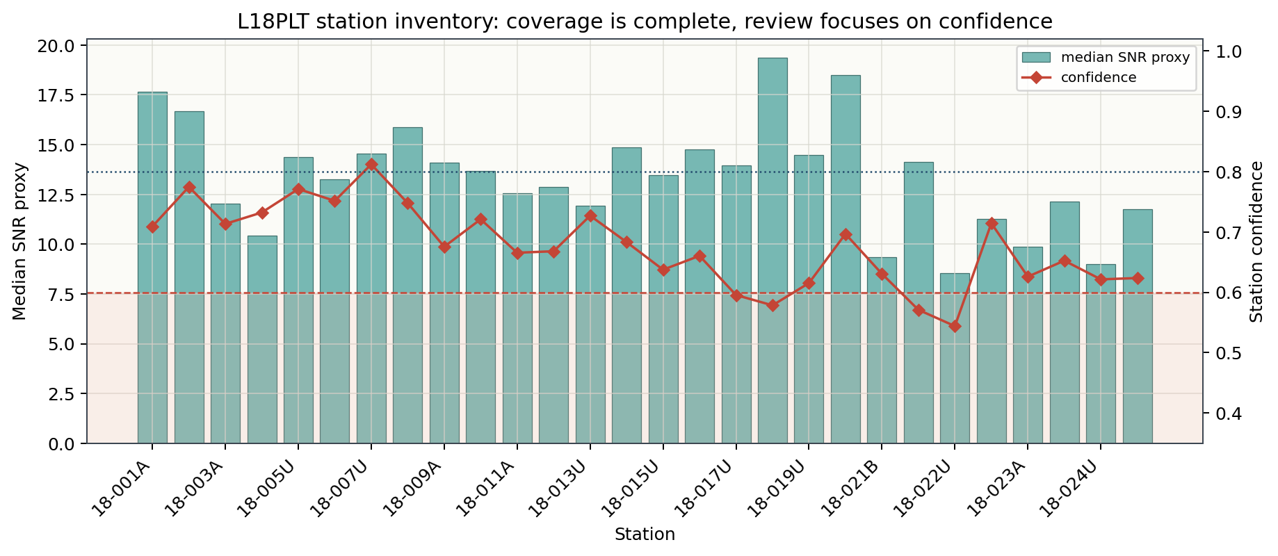
The SNR bars and the confidence line do not track each other station by station: the two tallest SNR bars on the line (around 18-019U and 18-021U) sit next to confidence dips, not peaks, while the single confidence value that clears the 0.80 line (18-007U, the only station in high_ci above) has an unremarkable, mid-range SNR bar. A higher SNR proxy describes signal strength relative to noise; it says nothing about tensor consistency, diagonal leakage, or spatial coherence, so it is not a substitute for the composite score.

The next two views show the same confidence logic in profile and period-frequency space:

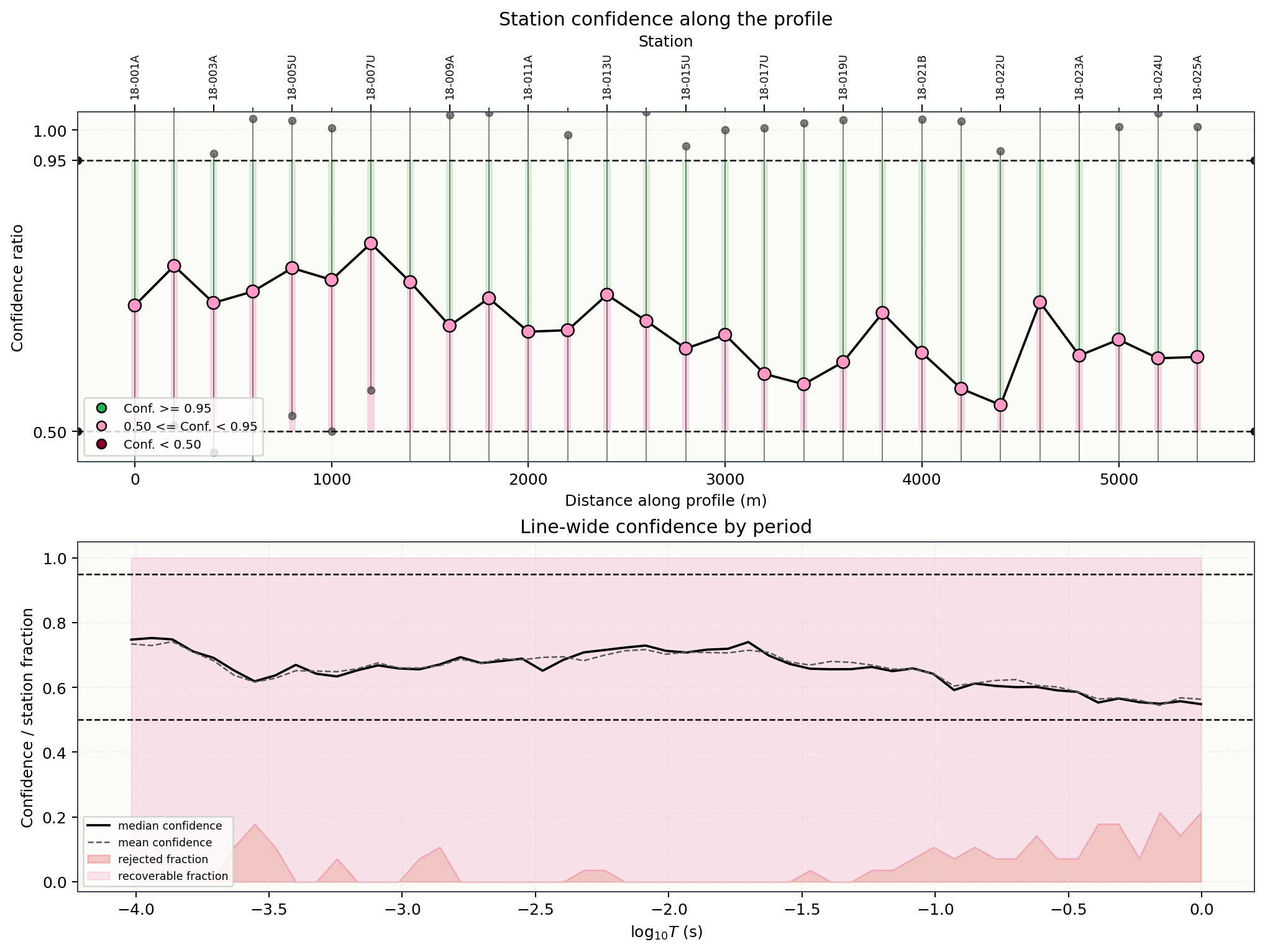
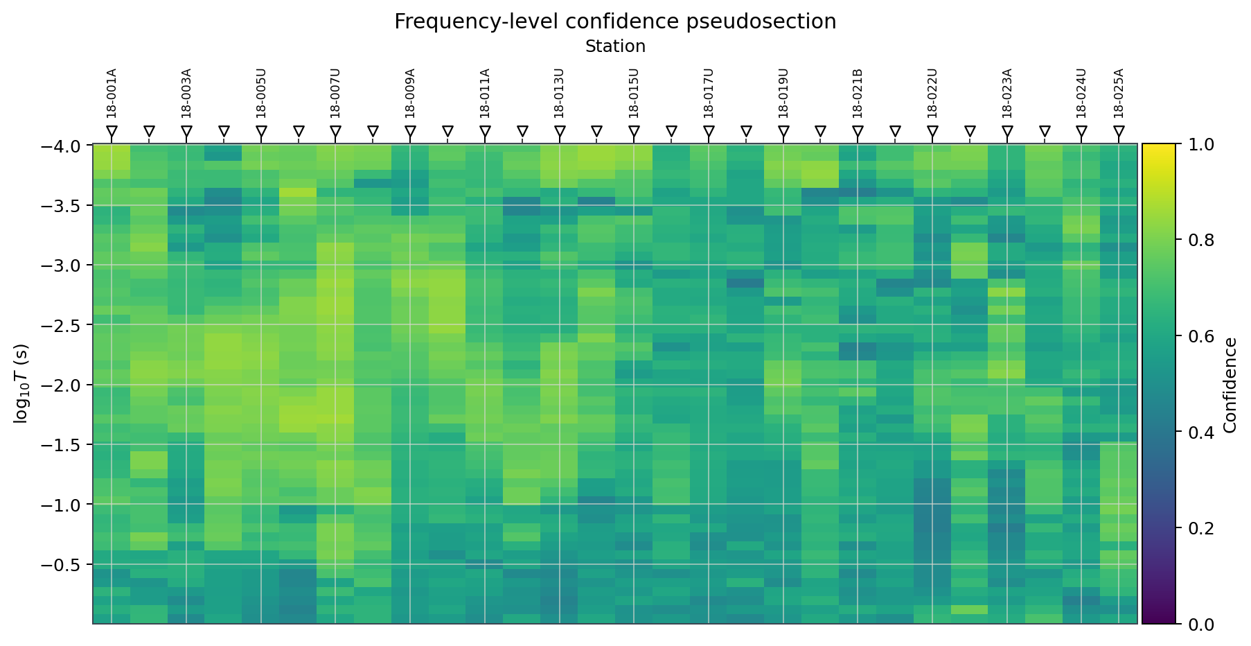
In the top-left panel, every station’s confidence marker falls in the pink 0.50-0.95 band – none reaches the green >= 0.95 tier anywhere along the 5.4 km profile, consistent with high_ci containing only one station. The bottom-left panel shows median and mean confidence declining gradually from about 0.75 at the shortest periods to about 0.55-0.6 at the longest, with the rejected-fraction band spiking at several scattered periods rather than one contiguous interval – a pattern more consistent with narrow-band noise recurring across the line than with a single missing or corrupted acquisition window. The right-hand pseudosection makes the same point spatially: confidence (viridis, yellow = high) is mostly uniform green-yellow, with the weak spots concentrated in vertical streaks at specific stations and short periods rather than smeared across the whole section – the same station-localized pattern already identified numerically above (18-021U, 18-013U, 18-021B, 18-022U, 18-023A), now visible directly rather than only in a table.

Use this plot to distinguish three common cases:

one or two isolated low-confidence stations, often worth manual repair
a continuous low-confidence interval, often worth comparing with geology, topography, and acquisition notes
profile-wide low confidence, often caused by import, rotation, unit, or configuration problems

L18PLT matches the first case: confidence problems cluster at a handful of identifiable stations and scattered periods rather than spreading evenly across the whole line, which is why this tutorial’s next steps (station lists, then Correct Static Shift) target specific stations instead of reprocessing the survey wholesale.

18.3.12. Select Stations for the Next Step#

After QC, create explicit station lists. This makes later correction and inversion runs easier to reproduce.

>>> keep_stations = (
...     station_ci_df.loc[station_ci_df["confidence"] >= 0.60, "station"]
...     .astype(str)
...     .tolist()
... )
>>> review_stations = (
...     station_ci_df.loc[station_ci_df["confidence"] < 0.60, "station"]
...     .astype(str)
...     .tolist()
... )
>>> len(keep_stations), len(review_stations)
(23, 5)
>>> _ = (qc_dir / "keep_stations.txt").write_text(
...     "\n".join(keep_stations) + "\n",
...     encoding="utf-8",
... )
>>> _ = (qc_dir / "review_stations.txt").write_text(
...     "\n".join(review_stations) + "\n",
...     encoding="utf-8",
... )

23 stations keep a confidence at or above the 0.60 review threshold and 5 fall below it – the same 5 stations identified in low_ci above. These lists can be used by later site selection, recomputation, static-shift correction, or inversion preparation steps.

18.3.13. CLI Quick Checks#

The Python API gives the richest QC tables. The CLI is useful for quick terminal checks before opening a notebook.

pycsamt edi info data/AMT/WILLY_DATA/L18PLT
pycsamt edi validate data/AMT/WILLY_DATA/L18PLT --deep
pycsamt site info data/AMT/WILLY_DATA/L18PLT --format csv > qc_review/site_inventory.csv
pycsamt site compute strike data/AMT/WILLY_DATA/L18PLT --format csv > qc_review/strike.csv
pycsamt site compute tipper data/AMT/WILLY_DATA/L18PLT --format csv > qc_review/tipper.csv

Use the CLI outputs as supporting diagnostics. Use the Python QC tables when you need confidence thresholds, frequency-level masking, or custom reporting.

18.3.14. What to Do With Poor Stations#

The QC result should lead to a processing decision. Common decisions are:

keep: The station has high confidence and acceptable frequency coverage.
review: The station has local problems but may be recoverable after frequency masking, component rotation, or static-shift analysis.
recompute: The station was exported by another program or has inconsistent component orientation, naming, or metadata. Use pyCSAMT site recomputation before modelling.
exclude from first trial: The station is too incomplete or unstable for the first inversion run. Keep it documented so it can be revisited after the first model explains the main survey response.

18.3.15. Troubleshooting#

No stations are loaded: Check the input path, file extension, and recursive=True when EDI files are inside line subdirectories.
All stations have low coverage: Inspect the EDI format and component names. The files may need recomputation or conversion before QC.
Confidence is low only at long periods: This may indicate noise, weak source field, dead-band behavior, or a real long-period response. Compare neighboring stations before masking.
Confidence is low only for one station: Check station coordinates, orientation, contact resistance notes, and whether the station was exported differently from the rest of the line.
Skew is high across a profile segment: Do not automatically delete those stations. Compare with structural geology, dimensionality diagnostics, and inversion residuals.

18.3.16. See Also#

Read an EDI Survey: Load EDI files and inspect the survey object.
Correct Static Shift: Apply a common first correction after QC.
Dimensionality, Distortion, And The Phase Tensor: Interpret high phase-tensor skew before assuming a 1-D/2-D structure.
EDI Recompute Workflow: Recompute and rewrite EDI files imported from external software.
Computed Diagnostics: Compute strike, resistivity, phase-slope, and tipper diagnostics.
pycsamt.emtools: EMTools API reference.