11.22. Gradient-Based Pseudo-Sections

pycsamt.emtools.gradient_imaging builds CSAMT/AMT apparent resistivity pseudo-sections from gradients rather than from resistivity values alone. The goal is boundary emphasis: highlight where apparent resistivity changes laterally, vertically, or in both directions at once.

The implementation follows the gradient apparent-resistivity ideas of Zhang, Farquharson, and Liu (2021). It is useful when a normal rho_a pseudo-section carries broad background variation that makes target boundaries difficult to see.

Full callable signatures live in the API reference. This page explains the quantities, returned tables, plotting workflow, component choices, and interpretation checks.

11.22.1. Why Use Gradients

A plain apparent-resistivity pseudo-section answers:

“How resistive is this station-frequency sample?”

A gradient pseudo-section answers a different question:

“Where does apparent resistivity change sharply?”

That difference matters in CSAMT/AMT interpretation. Boundary-like features can be clearer in derivatives than in raw values, especially when the background has broad smooth variation.

The method starts from a sampled apparent-resistivity surface \(\rho_a(x,T)\), where \(x\) is station position and \(T=1/f\) is period. The implemented quantities are finite differences on that sampled surface. They are not a substitute for an inversion model, but they are a useful way to make station-period boundaries visible before or alongside inversion.

11.22.2. The Three Quantities

The module computes apparent resistivity from impedance first. By default it uses the determinant-style geometric mean:

\[\rho_{xy} = 0.2 {|Z_{xy}|^2 \over f}, \qquad \rho_{yx} = 0.2 {|Z_{yx}|^2 \over f},\]

\[\rho_a = \sqrt{\rho_{xy}\rho_{yx}}.\]

You can also use one component only with comp="xy" or comp="yx".

The depth column is an apparent skin depth scale,

\[\delta = 503 \sqrt{\rho_a \over f},\]

reported in metres. It should be read as an approximate plotting depth, not as an inversion depth.

The three gradient products are:

Quantity	Meaning
spatial	Along-line station-to-station difference, \(\Delta\rho_a^x\).
frequency	Adjacent-frequency difference at each station, \(\Delta\rho_a^z\).
joint	Frequency difference of the spatial gradient, \(\Delta\rho_a^{zx}\).

The joint gradient is often the most useful image because it responds where the apparent resistivity changes both laterally and with frequency. Smooth background variation tends to be reduced.

11.22.3. Station Position And Spacing

The gradient tables need station order and station spacing. pyCSAMT uses station position metadata when available. If no usable coordinates are available, it falls back to regular spacing with spacing_m=200.0.

Always report the spacing assumption when using fallback spacing. The gradient values are apparent-resistivity differences, but the x-axis and pair spacing still affect interpretation of lateral scale.

For adjacent stations \(j-1\) and \(j\), the midpoint and spacing stored in the tables are

\[x_{j-1/2} = {x_{j-1}+x_j \over 2}, \qquad \Delta x_j = x_j - x_{j-1}.\]

The current tables report finite differences in ohm metres. If you need a normalized lateral derivative, divide delta_rho_x or delta_rho_zx by dx_m in your own workflow and state the resulting units.

11.22.4. Spatial Gradient

rho_spatial_gradient compares adjacent stations at the same frequency.

\[\Delta\rho_a^x(j, f) = \rho_a(x_j, f) - \rho_a(x_{j-1}, f).\]

The value is assigned to the midpoint between the two stations. Its sign is directional: positive means apparent resistivity increases to the right along the sorted line, while negative means it decreases.

>>> from pycsamt.emtools.gradient_imaging import rho_spatial_gradient
>>> spatial = rho_spatial_gradient(
...     "data/AMT/WILLY_DATA/L18PLT",
...     spacing_m=200.0,
...     comp="det",
... )
>>> spatial.head()
  station_a station_b    x_m  ...       depth_m   rho_a_ohmm  delta_rho_x
0   18-001A   18-002U  100.0  ...  16441.550076  1076.986058  -789.812389
1   18-001A   18-002U  100.0  ...  23164.458570  2553.493898   633.104370
2   18-001A   18-002U  100.0  ...  15708.445184  1402.456235  -407.796992
3   18-001A   18-002U  100.0  ...  16229.672127  1788.573047    68.027386
4   18-001A   18-002U  100.0  ...  22026.195330  3934.779127 -5968.395877
[5 rows x 9 columns]
>>> spatial.to_csv("l18plt_spatial_gradient.csv", index=False)

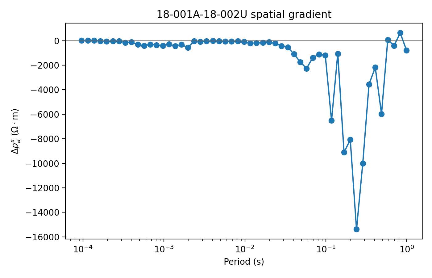
The full table holds every adjacent-station pair at every frequency. Plotting one pair’s gradient curve against period is a useful first look before assembling the full pseudo-section:

>>> import matplotlib.pyplot as plt
>>> pair = spatial.loc[spatial["station_a"] == "18-001A"].sort_values("period_s")
>>> fig, ax = plt.subplots(figsize=(7, 4.5))
>>> _ = ax.semilogx(pair["period_s"], pair["delta_rho_x"], "o-")
>>> _ = ax.axhline(0.0, color="0.4", linewidth=0.8)
>>> _ = ax.set_xlabel("Period (s)")
>>> _ = ax.set_ylabel(r"$\Delta\rho_a^x$ ($\Omega\cdot$m)")
>>> _ = ax.set_title("18-001A-18-002U spatial gradient")
>>> fig.tight_layout()

The output columns are:

• station_a and station_b: adjacent station pair.

• x_m: midpoint position of the pair.

• dx_m: station spacing for the pair.

• freq_hz and period_s: frequency and period.

• depth_m: skin-depth-style apparent depth at the pair.

• rho_a_ohmm: mean apparent resistivity of the station pair.

• delta_rho_x: lateral apparent-resistivity difference.

Positive delta_rho_x means the right station has higher apparent resistivity than the left station at that frequency. Negative values mean the opposite.

11.22.5. Frequency Gradient

rho_frequency_gradient compares adjacent frequencies at each station.

\[\Delta\rho_a^z(j, f_k) = \rho_a(x_j, f_k) - \rho_a(x_j, f_{k-1}).\]

The implementation uses the sorted frequency grid and assigns the result to the upper frequency \(f_k\). Because frequency and depth are linked only approximately, this is a frequency-direction contrast, not a true derivative with respect to physical depth.

>>> from pycsamt.emtools.gradient_imaging import rho_frequency_gradient
>>> vertical = rho_frequency_gradient(
...     "data/AMT/WILLY_DATA/L18PLT",
...     spacing_m=200.0,
...     comp="det",
... )
>>> one = vertical.loc[vertical["station"] == "18-001A"].sort_values("period_s")
>>> one[["period_s", "rho_a_ohmm", "delta_rho_z"]].head()
   period_s  rho_a_ohmm  delta_rho_z
51  0.000096   80.630809    -7.264990
50  0.000115   86.503532    -4.480456
49  0.000137  102.020596   -26.553673
48  0.000164  133.745279   -36.895692
47  0.000196  154.026762    -3.667275

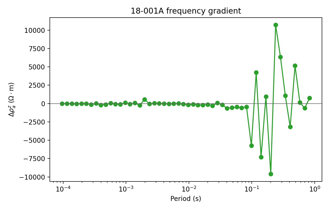
Plotting the same station’s full curve against period shows where the sign flips and how it grows toward the low-frequency end:

>>> fig, ax = plt.subplots(figsize=(7, 4.5))
>>> _ = ax.semilogx(one["period_s"], one["delta_rho_z"], "o-", color="C2")
>>> _ = ax.axhline(0.0, color="0.4", linewidth=0.8)
>>> _ = ax.set_xlabel("Period (s)")
>>> _ = ax.set_ylabel(r"$\Delta\rho_a^z$ ($\Omega\cdot$m)")
>>> _ = ax.set_title("18-001A frequency gradient")
>>> fig.tight_layout()

The output columns are:

• station: station name.

• x_m: station position.

• freq_hz and period_s: upper frequency of the adjacent pair.

• depth_m: apparent depth at the mean resistivity of the pair.

• rho_a_ohmm: mean apparent resistivity of the two frequencies.

• delta_rho_z: frequency-direction apparent-resistivity difference.

This quantity is a proxy for vertical or depth-related changes because different frequencies sample different investigation depths.

11.22.6. Joint Gradient

rho_joint_gradient computes the frequency difference of the spatial gradient.

\[\Delta\rho_a^{zx}(j, f_k) = \Delta\rho_a^x(j, f_k) - \Delta\rho_a^x(j, f_{k-1})\]

Expanded:

\[\Delta\rho_a^{zx}(j, f_k) = [\rho_a(j, f_k) - \rho_a(j-1, f_k)] - [\rho_a(j, f_{k-1}) - \rho_a(j-1, f_{k-1})]\]

This is a mixed finite difference on the station-frequency grid:

\[\Delta\rho_a^{zx} = \Delta_f\left(\Delta_x\rho_a\right).\]

>>> from pycsamt.emtools.gradient_imaging import rho_joint_gradient
>>> joint = rho_joint_gradient(
...     "data/AMT/WILLY_DATA/L18PLT",
...     spacing_m=200.0,
...     comp="det",
... )
>>> joint.head()
  station_a station_b    x_m  ...  period_s       depth_m  delta_rho_zx
0   18-001A   18-002U  100.0  ...  0.830565  19740.513225   1422.916759
1   18-001A   18-002U  100.0  ...  0.695410  18387.618571  -1040.901362
2   18-001A   18-002U  100.0  ...  0.582072  15731.499213    475.824378
3   18-001A   18-002U  100.0  ...  0.487329  14850.211800  -6036.423263
4   18-001A   18-002U  100.0  ...  0.407997  16531.998598   3783.198291
[5 rows x 8 columns]
>>> joint.to_csv("l18plt_joint_gradient.csv", index=False)

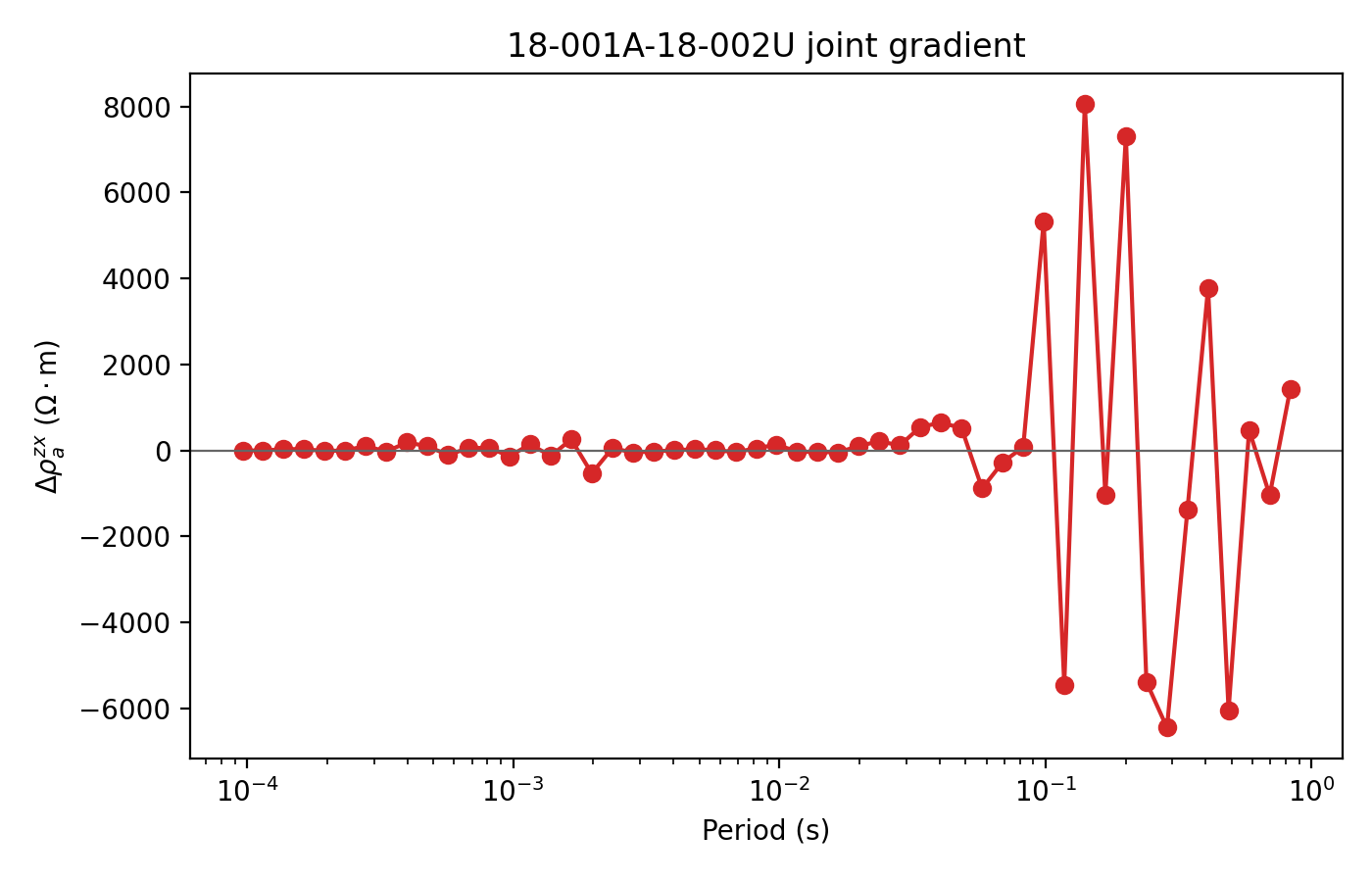
The same pair’s joint gradient, sorted by period, mixes the spatial and frequency contrasts together:

>>> pair_joint = joint.loc[joint["station_a"] == "18-001A"].sort_values("period_s")
>>> fig, ax = plt.subplots(figsize=(7, 4.5))
>>> _ = ax.semilogx(pair_joint["period_s"], pair_joint["delta_rho_zx"], "o-", color="C3")
>>> _ = ax.axhline(0.0, color="0.4", linewidth=0.8)
>>> _ = ax.set_xlabel("Period (s)")
>>> _ = ax.set_ylabel(r"$\Delta\rho_a^{zx}$ ($\Omega\cdot$m)")
>>> _ = ax.set_title("18-001A-18-002U joint gradient")
>>> fig.tight_layout()

The output columns are:

• station_a and station_b: adjacent station pair.

• x_m: midpoint position of the pair.

• dx_m: station spacing for the pair.

• freq_hz and period_s: upper frequency of the adjacent frequency pair.

• depth_m: apparent depth from the median resistivity of the four surrounding station-frequency cells.

• delta_rho_zx: joint frequency-spatial gradient.

Joint gradients are strongest when lateral contrast changes with frequency. That is why they are useful for boundary delineation.

11.22.7. Plot Gradient Sections

plot_gradient_section is the main visualization helper. It accepts quantity="spatial", "frequency", or "joint".

The plotted grid is assembled as

\[G_{i,j} = q(T_i, x_j),\]

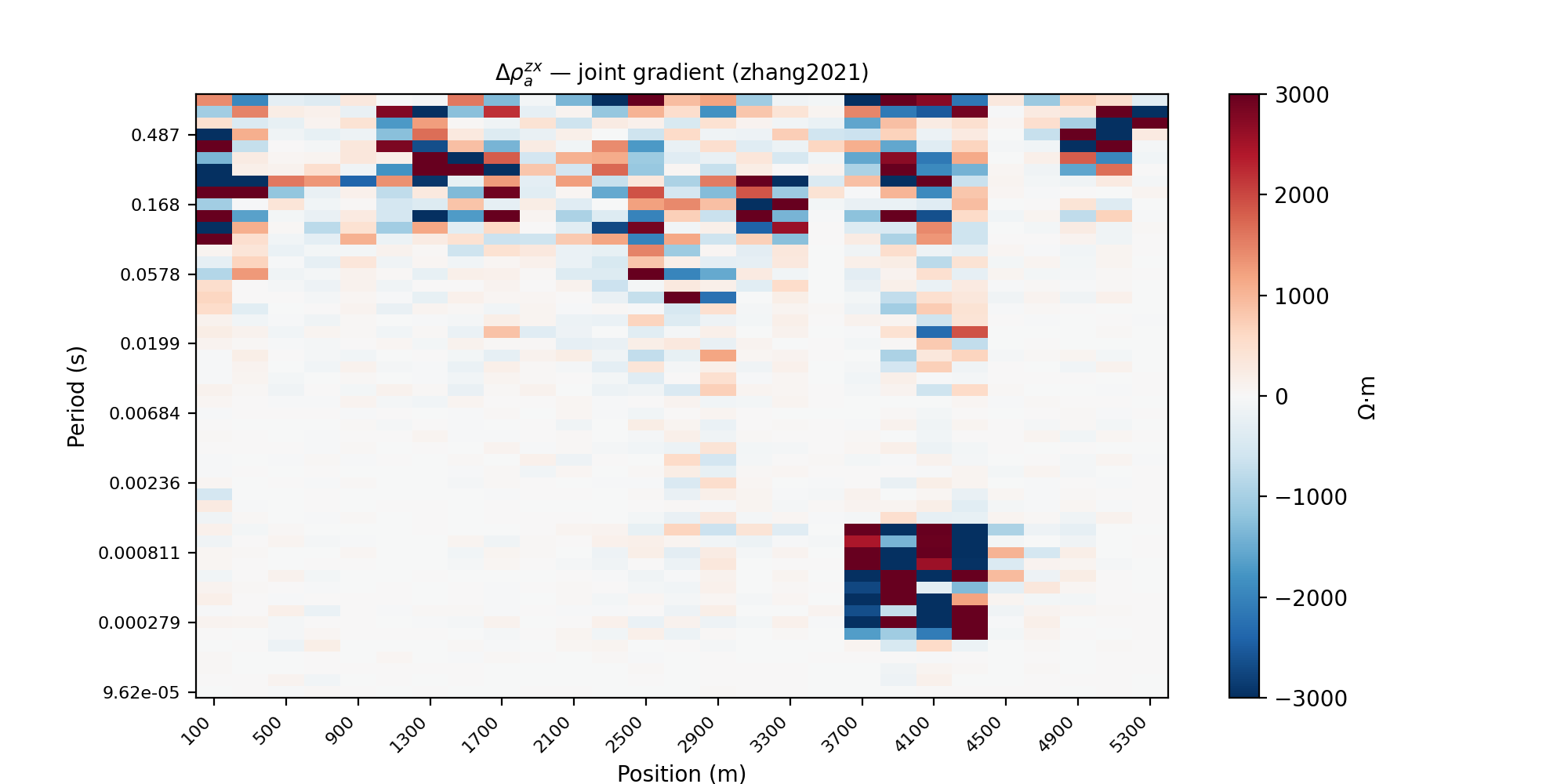
where \(q\) is one of \(\Delta\rho_a^x\), \(\Delta\rho_a^z\), or \(\Delta\rho_a^{zx}\). A diverging color map centered at zero is used because zero means “no local change” for the selected finite difference, while the sign tells the direction of the contrast.

>>> import matplotlib.pyplot as plt
>>> from pycsamt.emtools.gradient_imaging import plot_gradient_section
>>> survey = "data/AMT/WILLY_DATA/L18PLT"
>>> fig, axes = plt.subplots(1, 3, figsize=(15, 5), sharey=True)
>>> _ = plot_gradient_section(survey, quantity="spatial", ax=axes[0])
>>> _ = axes[0].set_title("Spatial")
>>> _ = plot_gradient_section(survey, quantity="frequency", ax=axes[1])
>>> _ = axes[1].set_title("Frequency")
>>> _ = plot_gradient_section(survey, quantity="joint", ax=axes[2])
>>> _ = axes[2].set_title("Joint")
>>> fig.tight_layout()

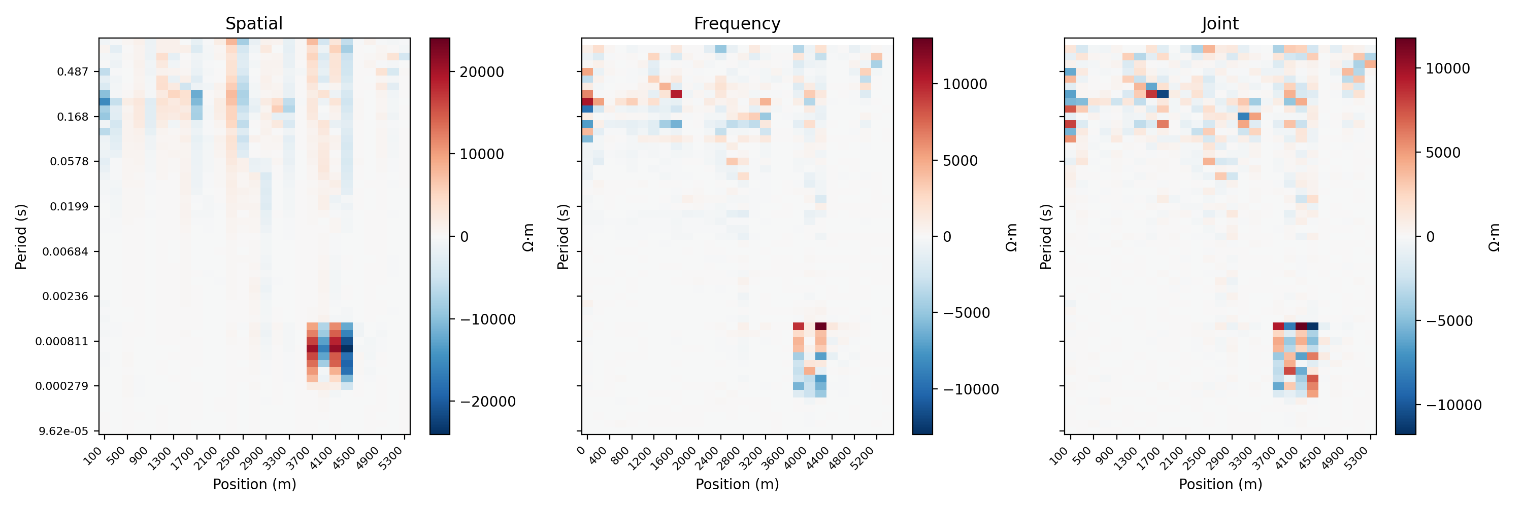
The color map is centered at zero by default. Positive and negative gradients are both meaningful: they indicate opposite directions of apparent-resistivity change.

Use vlim when comparing several lines or components so the color scale is consistent.

>>> from pycsamt.emtools.gradient_imaging import plot_gradient_section
>>> ax = plot_gradient_section(
...     "data/AMT/WILLY_DATA/L18PLT",
...     quantity="joint",
...     comp="det",
...     vlim=(-3000.0, 3000.0),
... )

11.22.8. Choosing The Impedance Component

All gradient functions accept:

comp	Meaning
"det"	Geometric mean of xy and yx apparent resistivities.
"xy"	Use only Zxy.
"yx"	Use only Zyx.

The default "det" is usually more stable because it combines both off-diagonal modes. Component-specific plots are still important when the two modes disagree.

>>> import pandas as pd
>>> from pycsamt.emtools.gradient_imaging import rho_joint_gradient
>>> survey = "data/AMT/WILLY_DATA/L18PLT"
>>> rows = []
>>> for comp in ("det", "xy", "yx"):
...     table = rho_joint_gradient(survey, comp=comp)
...     rows.append(
...         {
...             "component": comp,
...             "std": table["delta_rho_zx"].std(),
...             "max_abs": table["delta_rho_zx"].abs().max(),
...         }
...     )
...
>>> component_sensitivity = pd.DataFrame(rows)
>>> component_sensitivity
  component          std        max_abs
0       det  1204.168366   11797.378008
1        xy  2574.547370   32488.264297
2        yx  9243.952423  175431.466235

Report the component whenever you show a gradient section.

11.22.9. Single-Pair And Single-Station Curves

Before interpreting a full pseudo-section, inspect a station pair or station curve.

>>> from pycsamt.emtools.gradient_imaging import (
...     rho_frequency_gradient,
...     rho_spatial_gradient,
... )
>>> survey = "data/AMT/WILLY_DATA/L18PLT"
>>> spatial = rho_spatial_gradient(survey)
>>> pair = spatial.loc[spatial["station_a"] == "18-001A"].sort_values("period_s")
>>> frequency = rho_frequency_gradient(survey)
>>> station = frequency.loc[frequency["station"] == "18-001A"].sort_values("period_s")
>>> fig, (ax_pair, ax_station) = plt.subplots(2, 1, figsize=(7, 7), sharex=True)
>>> _ = ax_pair.semilogx(pair["period_s"], pair["delta_rho_x"], "o-")
>>> _ = ax_pair.axhline(0.0, color="0.4", linewidth=0.8)
>>> _ = ax_pair.set_ylabel("Spatial gradient")
>>> _ = ax_station.semilogx(station["period_s"], station["delta_rho_z"], "o-", color="C2")
>>> _ = ax_station.axhline(0.0, color="0.4", linewidth=0.8)
>>> _ = ax_station.set_xlabel("Period (s)")
>>> _ = ax_station.set_ylabel("Frequency gradient")
>>> fig.tight_layout()

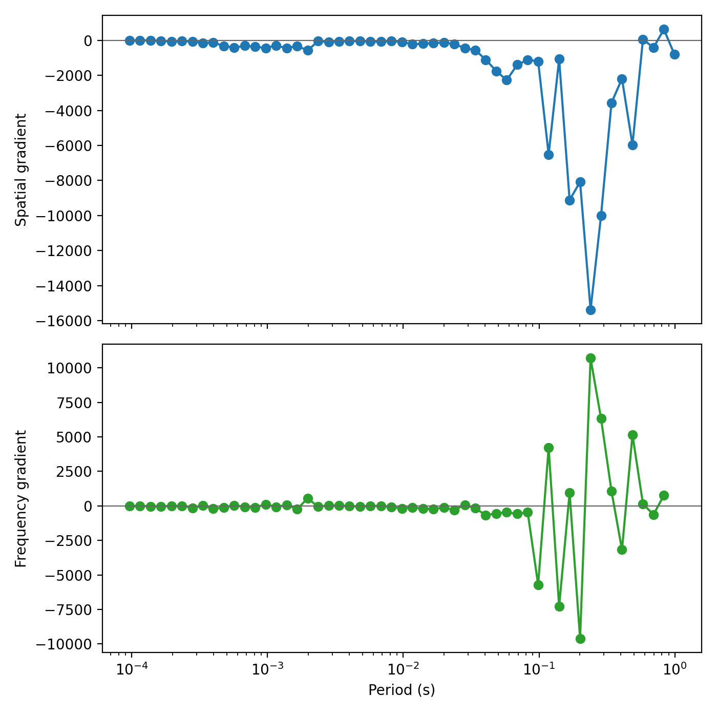
This makes it easier to tell whether a pseudo-section hotspot comes from one extreme station pair, one frequency jump, or a coherent region.

11.22.10. Does The Joint Gradient Suppress Background?

One practical check is to compare the spread of the spatial and joint gradients. A joint gradient that is quieter in background areas should often have a narrower distribution, while preserving strong localized values.

The reported ratio is

\[R = {\operatorname{std}(\Delta\rho_a^{zx}) \over \operatorname{std}(\Delta\rho_a^x)}.\]

Values below one mean the joint gradient is globally narrower than the spatial gradient. That supports, but does not prove, the idea that background variation has been reduced.

>>> from pycsamt.emtools.gradient_imaging import (
...     rho_joint_gradient,
...     rho_spatial_gradient,
... )
>>> survey = "data/AMT/WILLY_DATA/L18PLT"
>>> spatial = rho_spatial_gradient(survey)
>>> joint = rho_joint_gradient(survey)
>>> spatial_std = spatial["delta_rho_x"].std()
>>> joint_std = joint["delta_rho_zx"].std()
>>> print(f"spatial std = {spatial_std:.1f} ohm.m")
spatial std = 2200.1 ohm.m
>>> print(f"joint std   = {joint_std:.1f} ohm.m")
joint std   = 1204.2 ohm.m
>>> print(f"ratio       = {joint_std / spatial_std:.2f}")
ratio       = 0.55

This is not a proof of geological correctness, but it is a useful sanity check before relying on the joint image.

11.22.11. Compare Neighboring Lines

Use the same quantity, comp, and vlim when comparing lines.

>>> from pycsamt.emtools.gradient_imaging import plot_gradient_section
>>> l18 = "data/AMT/WILLY_DATA/L18PLT"
>>> l22 = "data/AMT/WILLY_DATA/L22PLT"
>>> fig, (ax18, ax22) = plt.subplots(1, 2, figsize=(13, 5), sharey=True)
>>> _ = plot_gradient_section(l18, quantity="joint", comp="det", vlim=(-3000, 3000), ax=ax18)
>>> _ = ax18.set_title("L18PLT")
>>> _ = plot_gradient_section(l22, quantity="joint", comp="det", vlim=(-3000, 3000), ax=ax22)
>>> _ = ax22.set_title("L22PLT")
>>> fig.tight_layout()

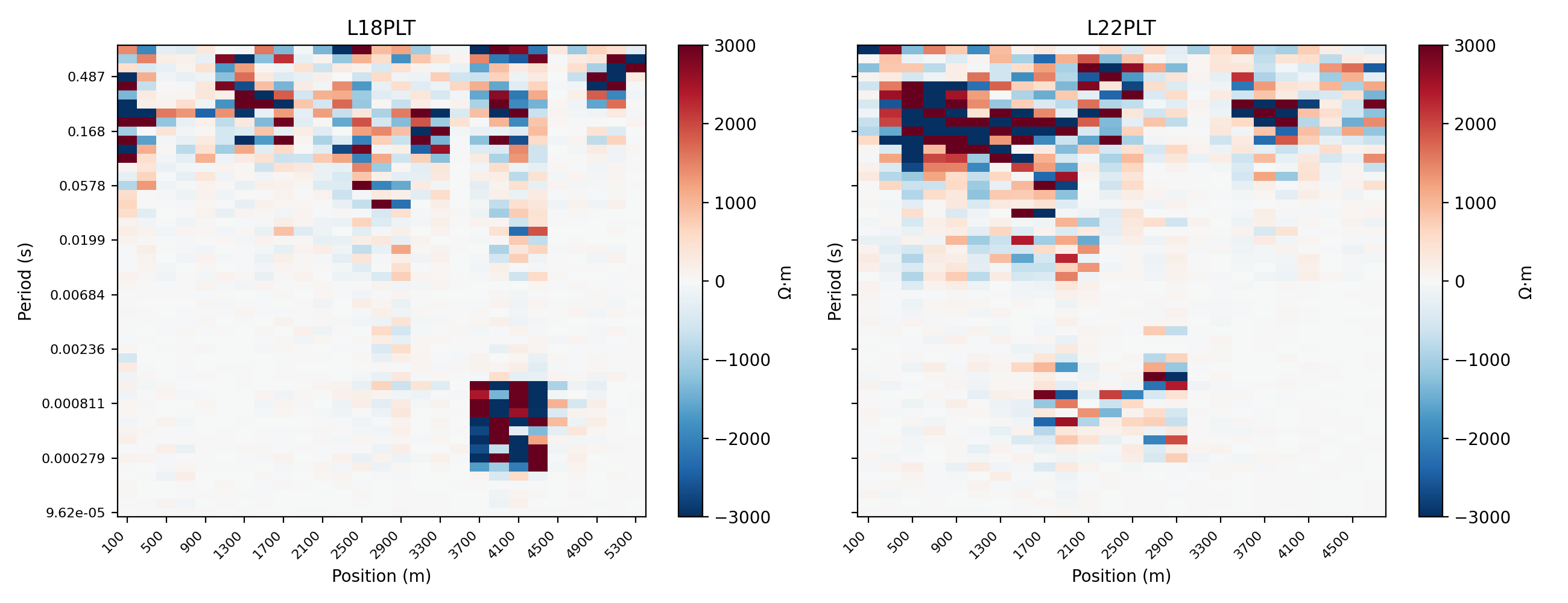
Line-to-line similarity is a useful processing sanity check. Differences can still be geological, but first confirm the same band, component, and color scale were used.

11.22.12. Reading The Results

Use this interpretation order:

• Start with comp="det" for a stable overview.

• Check xy and yx separately when off-diagonal modes disagree.

• Use the spatial gradient for lateral station-to-station contrasts.

• Use the frequency gradient for single-station vertical changes.

• Use the joint gradient for features that are both lateral and depth-dependent.

• Prefer coherent station-period regions over isolated extreme cells.

• Compare neighboring lines with the same vlim before making a structural interpretation.

11.22.13. Common Failure Modes

Missing or irregular station positions

The module falls back to spacing_m. Report the assumed spacing when coordinates are unavailable.

Component-driven artifacts

xy and yx can behave very differently. Always record comp and inspect determinant vs component-specific results.

Over-reading sign

Positive and negative gradients indicate direction of change. A boundary can appear as adjacent positive and negative lobes.

Noisy frequency rows

Gradients amplify row-to-row changes. Run frequency QC before interpreting subtle gradient features.

Color-scale mismatch

Automatic color limits can make two lines look more different or more similar than they are. Use fixed vlim for comparisons.

11.22.14. Saving A Reproducible Bundle

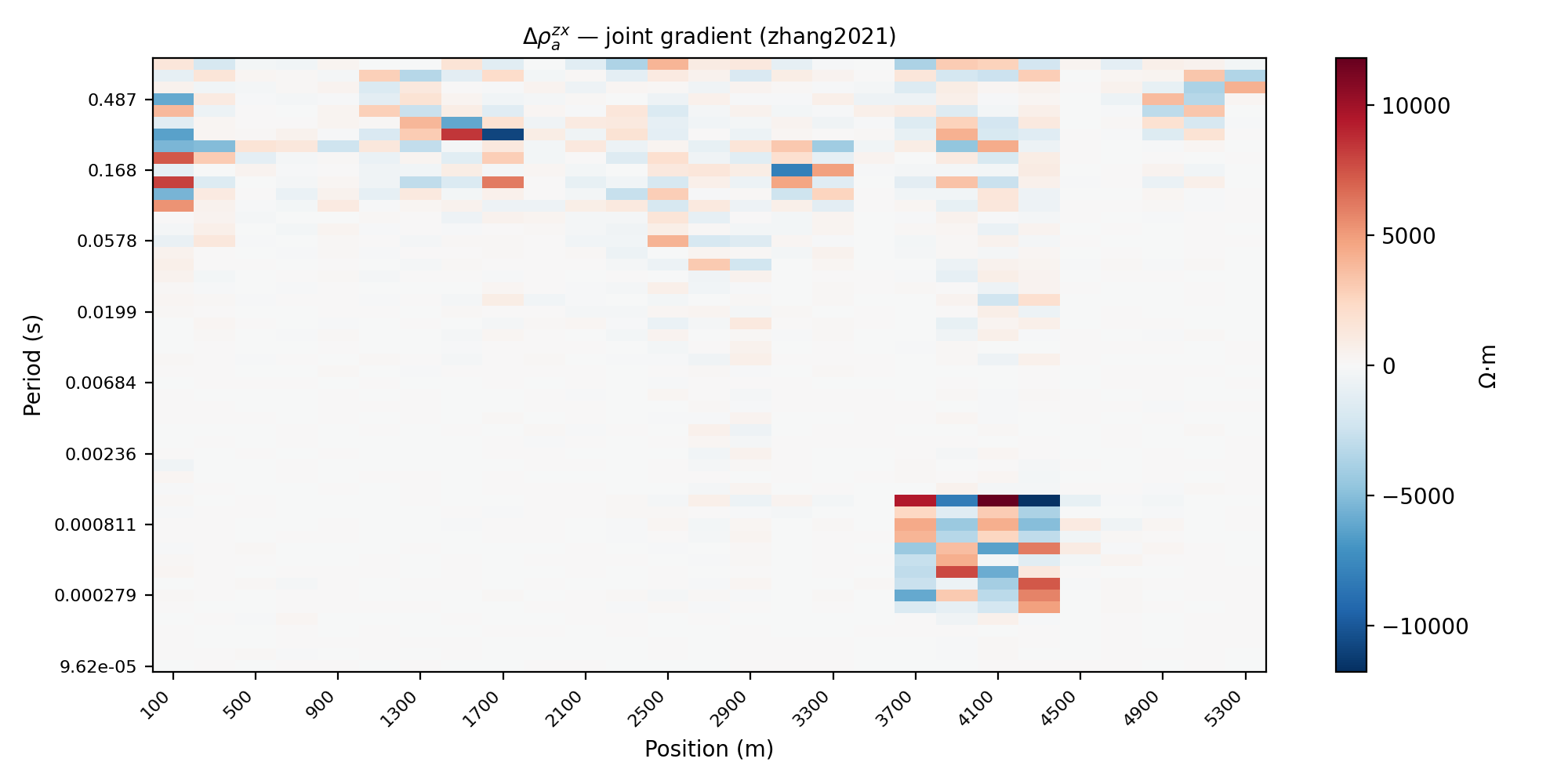
Save the three gradient tables and the main pseudo-section.

>>> from pathlib import Path
>>> from pycsamt.emtools.gradient_imaging import (
...     plot_gradient_section,
...     rho_frequency_gradient,
...     rho_joint_gradient,
...     rho_spatial_gradient,
... )
>>> survey = "data/AMT/WILLY_DATA/L18PLT"
>>> out = Path("outputs/gradient_l18plt")
>>> out.mkdir(parents=True, exist_ok=True)
>>> spatial = rho_spatial_gradient(survey, comp="det")
>>> frequency = rho_frequency_gradient(survey, comp="det")
>>> joint = rho_joint_gradient(survey, comp="det")
>>> spatial.to_csv(out / "spatial_gradient.csv", index=False)
>>> frequency.to_csv(out / "frequency_gradient.csv", index=False)
>>> joint.to_csv(out / "joint_gradient.csv", index=False)
>>> fig, ax = plt.subplots(figsize=(10, 5))
>>> _ = plot_gradient_section(survey, quantity="joint", comp="det", ax=ax)
>>> fig.tight_layout()
>>> fig.savefig(out / "joint_gradient_section.png", dpi=200)

11.22.15. Worked Example

The gallery example uses L18PLT and compares it with neighboring L22PLT from data/AMT/WILLY_DATA/. It demonstrates one station pair, one station frequency-gradient curve, the joint gradient, all three pseudo-sections, background-suppression checks, component sensitivity, and line-to-line comparison.

Open the rendered example here: Gradient-based CSAMT pseudo-sections (pycsamt.emtools.gradient_imaging).