6.3.16. AI inversion validation#

Validation determines whether an AI inversion model is fit for a stated use, not merely whether it can predict a synthetic test array. A defensible result must be accurate in parameter space, reproduce the electromagnetic response, remain stable under realistic perturbations, behave honestly when uncertain, and add value relative to a simpler baseline model or to an established classical inversion.

This page provides a validation protocol for models trained as described in Training AI inversion models. Uncertainty calibration is treated in AI inversion uncertainty, while the final evidence package is assembled in AI inversion reporting.

6.3.16.1. Validation is a claim with a scope#

Write the intended-use statement before computing metrics. It is the domain condition attached to every number that follows. If a fitted model is represented by \(g_\theta\) and the measured feature vector by \(\mathbf{x}\), validation is not the unconditional claim that \(g_\theta(\mathbf{x})\) is correct everywhere. It is the narrower claim that, for samples drawn from a declared domain \(\mathcal{D}\), the prediction \(\hat{\mathbf{m}} = g_\theta(\mathbf{x})\) is accurate enough for a named decision and fails visibly outside that domain. The statement should name:

survey method and components, such as AMT, MT, apparent resistivity, and phase;
frequency range, station spacing, and expected data-quality range;
geological families and resistivity contrasts represented;
output dimensionality, layer count, depth range, and parameter units;
whether the result is for screening, initialization, interpretation, or a decision requiring quantitative accuracy;
conditions under which the model must abstain or be reviewed.

A model validated for five-layer synthetic 1D earths is not thereby validated for a strongly 3D field setting. Every acceptance statement should be read as “validated for this declared domain under these tests.”

6.3.16.2. The evaluation partitions#

Keep the roles of data partitions distinct:

training: Updates model weights.
validation: Controls early stopping, architecture choice, and hyperparameters.
calibration: Fits conformal or posterior calibration when required.
test: Measures final performance after all choices are frozen.
challenge: Optional deliberately shifted cases used to identify failure boundaries.

The calibration set and challenge set have different jobs. A calibration set adjusts uncertainty statements after the model architecture is chosen; a challenge set maps the failure boundary and should not quietly become a source of tuning decisions. The test set is not a second validation set. If its results cause another round of tuning, it has become development data and a new untouched test set is required.

Split by independent geological realization or survey, not merely by row. Noise variants from one forward model, overlapping profile windows, or nodes from one synthetic graph must remain in the same partition. Record the split manifest and verify that parent identifiers do not cross boundaries. Any path by which held-out information influences model selection, preprocessing, or threshold setting is validation leakage; it usually makes the final score optimistic in a way that is difficult to repair after the fact.

Important

The current high-level supervised trainers estimate normalization statistics before making their internal training/validation split. This limitation affects the internal validation curve. It does not justify exposing the external test set: keep test and calibration arrays entirely outside fit and document the preprocessing behavior in the evidence report.

6.3.16.3. Freeze the artifact before testing#

Before opening the test set, preserve:

model checkpoint and checksum;
configuration and random seeds;
dataset and split identifiers;
preprocessing and target transforms;
pyCSAMT, backend, Python, and dependency versions;
selected epoch and selection rationale;
acceptance thresholds written without reference to test results.

Reload the checkpoint in a fresh process and reproduce a small reference prediction. This catches missing normalizers, incompatible shapes, and serialization assumptions before scientific evaluation begins.

6.3.16.4. Parameter-space evaluation#

For 1-D inversion, request predictions in the same representation as the stored targets. The default output of pycsamt.ai.inversion.EMInverter1D.predict() contains logarithmic resistivity and, when log_thickness=True, logarithmic thickness.

Model-space metric values are easiest to audit when each target quantity keeps its own units. For sample \(i\) and layer \(\ell\), let \(y^{\rho}_{i\ell}=\log_{10}\rho_{i\ell}\) and \(\hat{y}^{\rho}_{i\ell}\) be the predicted log-resistivity. The log-space error is \(e^{\rho}_{i\ell}=\hat{y}^{\rho}_{i\ell}-y^{\rho}_{i\ell}\), while the corresponding multiplicative physical error is \(10^{|e^{\rho}_{i\ell}|}\). If \(\mathcal{M}\) is the finite-value mask for the entries included in a metric, the masked RMSE is

(1)#\[\operatorname{RMSE} = \sqrt{ \frac{1}{|\mathcal{M}|} \sum_{(i,j)\in\mathcal{M}} \left(\hat{y}_{ij}-y_{ij}\right)^2 }.\]

Equation (1) is meaningful only with its mask, target representation, and units. A trained workflow would call inverter.predict(X_test, as_log_rho=True). The miniature example below isolates the metric semantics with fixed arrays so the reported output is reproducible:

>>> import numpy as np
>>> from pycsamt.ai.training.metrics import layer_rmse, summarise
>>>
>>> n_layers = 3
>>> y_test = np.array([
...     [2.0, 2.5, 3.0, 60.0, 120.0],
...     [2.3, 2.8, 3.2, 80.0, 160.0],
...     [1.9, 2.4, 2.9, np.nan, 140.0],
... ])
>>> y_pred = np.array([
...     [2.1, 2.4, 3.1, 65.0, 110.0],
...     [2.2, 2.9, 3.1, 90.0, 150.0],
...     [2.0, 2.5, 3.0, 75.0, 135.0],
... ])
>>>
>>> overall = summarise(y_test, y_pred, n_layers=n_layers)
>>> per_parameter = layer_rmse(y_test, y_pred)
>>> {name: round(value, 4) for name, value in overall.items()}
{'rmse': 5.0006, 'mae': 2.9214, 'r2': 0.9923, 'relative_rmse': 0.0596, 'depth_rmse': 0.0577}
>>> print("resistivity RMSE by layer:", np.round(per_parameter[:n_layers], 4))
resistivity RMSE by layer: [0.1 0.1 0.1]
>>> print("thickness RMSE by interface:", np.round(per_parameter[n_layers:], 4))
thickness RMSE by interface: [7.9057 8.6603]
>>> print("finite target values:", int(np.isfinite(y_test).sum()))
finite target values: 14

The available metric helpers ignore non-finite entries. Report how many values each metric used; a score based on a small surviving fraction can look misleadingly good.

Interpret metrics in their actual space:

RMSE and MAE: Express typical error magnitude. In log10 resistivity, an absolute error of 0.3 corresponds to approximately a factor of two, not 0.3 ohm-m.
R-squared: Compares residual variation with target variation. It can be negative and can look strong when broad target ranges dominate scientifically important local errors.
Relative RMSE: Divides errors by target magnitude. It becomes unstable near zero and is awkward for log-valued targets, so do not use it without explaining the representation.
Depth-weighted RMSE: Summarizes resistivity errors with layer-index weighting. The current helper gives deeper layers less influence; it does not replace explicit depth-resolved results.

The first scalar RMSE in the example is intentionally poor as a headline number: it mixes log-resistivity entries and metre-valued thickness entries. Never combine resistivity and thickness into one headline score without also showing their separate physical-unit errors. Convert predictions back to ohm-m and metres for decision-facing tables:

>>> rho_true = 10.0 ** y_test[:, :n_layers]
>>> rho_pred = 10.0 ** y_pred[:, :n_layers]
>>> h_true = y_test[:, n_layers:]
>>> h_pred = y_pred[:, n_layers:]
>>>
>>> rho_factor_error = np.maximum(rho_pred / rho_true, rho_true / rho_pred)
>>> thickness_abs_error = np.abs(h_pred - h_true)
>>> print("median rho factor error:", np.round(np.nanmedian(rho_factor_error, axis=0), 3))
median rho factor error: [1.259 1.259 1.259]
>>> print("median thickness abs error m:", np.round(np.nanmedian(thickness_abs_error, axis=0), 3))
median thickness abs error m: [ 7.5 10. ]
>>> print("worst rho factor error:", round(float(np.nanmax(rho_factor_error)), 3))
worst rho factor error: 1.259

Report medians, upper quantiles, and worst credible cases in addition to means. Aggregate metrics should be broken down by layer, cumulative interface depth, resistivity contrast, conductor thickness, and data quality.

6.3.16.5. Model geometry and boundary recovery#

Layered targets need geometry-aware diagnostics. Compute interface depths by cumulatively summing thicknesses for every sample, \(z_{ik}=\sum_{\ell=1}^{k}h_{i\ell}\), where \(h_{i\ell}\) is layer thickness and \(z_{ik}\) is the depth to interface \(k\). Then evaluate:

interface-depth absolute and relative error;
whether important conductive or resistive units are detected;
top and base depth error for target units;
resistivity-thickness trade-offs;
false layers, merged layers, and missed thin layers;
performance as interfaces approach the investigation limit.

For 2-D and 3-D outputs, report cell-wise error together with structural measures: lateral boundary position, depth extent, connected-body recovery, and smoothing or edge artifacts. A low image RMSE can coexist with a badly placed target boundary.

The aggregation trap is observable, not theoretical#

The next audit constructs two 2-D predictions with the same global RMSE. One misplaces the target conductor; the other adds spatially correlated error throughout the section. Both are evaluated by recovery_report() without post-processing:

shifted conductor: RMSE=0.3832  MAE=0.1001  SSIM=0.7683
diffuse error:     RMSE=0.3832  MAE=0.2995  SSIM=0.3265

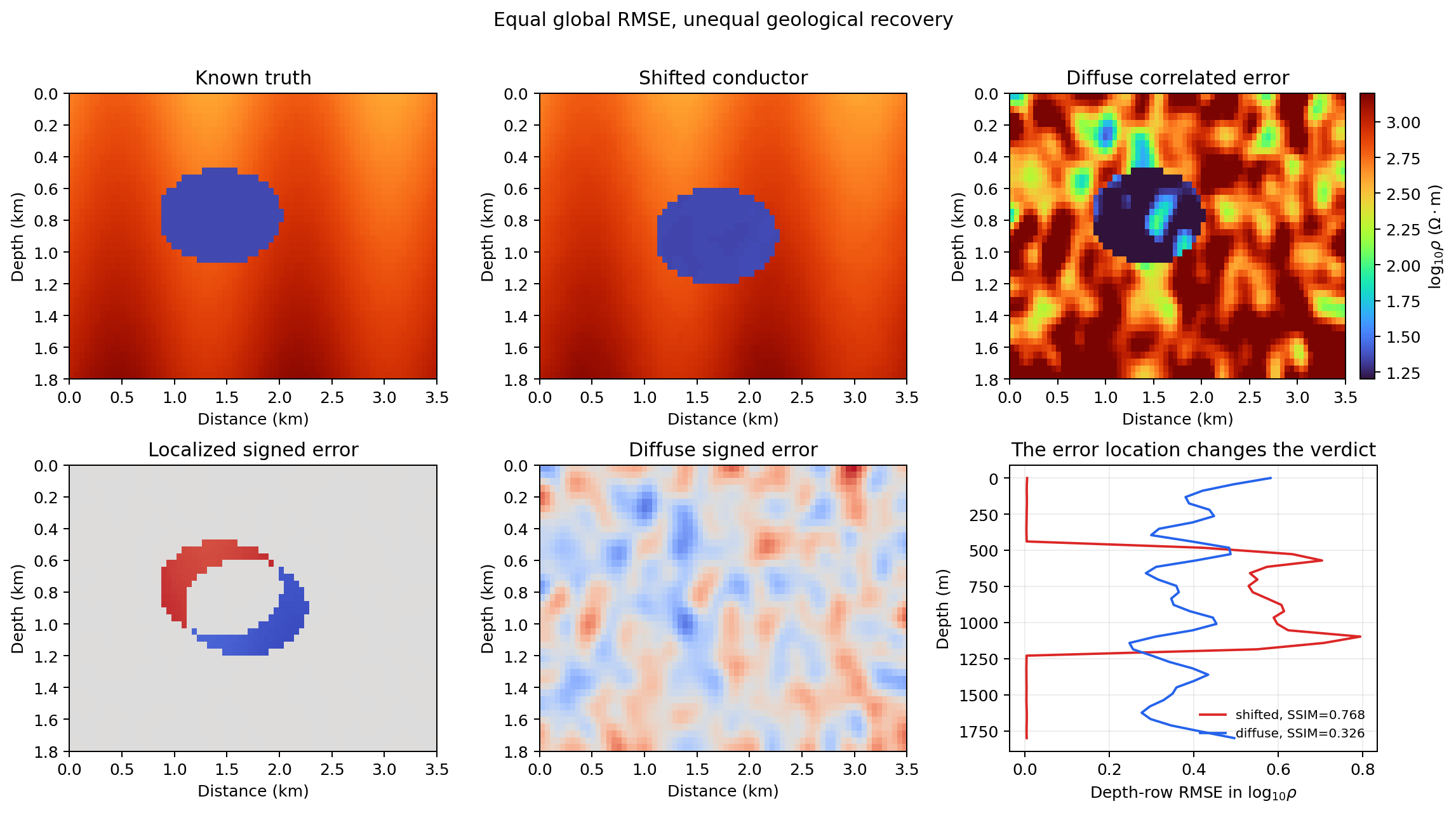
Known resistivity truth compared with a shifted conductor and diffuse correlated error having equal global RMSE, followed by signed errors and depth-resolved RMSE — Equal global RMSE engineered to machine precision, then assessed through structure and depth rather than accepted as equivalent.#

The shifted-conductor prediction concentrates a large signed error around one geological boundary, yet its low-error background yields much lower MAE and higher structural similarity than the diffuse prediction. Whether that is the better model depends on intended use: it may be preferable for regional background resistivity but unacceptable if locating the conductor is the decision. The depth curves reveal where each failure occurs. A scalar gate cannot encode that distinction, so pair global recovery with target-boundary, depth-resolved, and response-space gates chosen before testing.

View and copy the equal-RMSE recovery auditClick to inspect and copy the complete code

def make_validation_aggregation_trap() -> None:
    """Show why equal global RMSE does not imply equal earth recovery."""
    from scipy.ndimage import gaussian_filter

    from pycsamt.ai.validation import recovery_report

    rng = np.random.default_rng(90210)
    nz, nx = 42, 72
    z = np.linspace(0, 1, nz)[:, None]
    x = np.linspace(-1, 1, nx)[None, :]
    truth = 2.7 + 0.35 * z + 0.10 * np.sin(2 * np.pi * x)
    conductor = ((x + 0.18) / 0.34) ** 2 + ((z - 0.43) / 0.17) ** 2 <= 1
    truth = np.where(conductor, 1.35, truth)

    shifted_mask = ((x + 0.04) / 0.34) ** 2 + ((z - 0.50) / 0.17) ** 2 <= 1
    localized = np.where(shifted_mask, 1.35, 2.7 + 0.35 * z + 0.10 * np.sin(2 * np.pi * x))
    localized += gaussian_filter(rng.normal(scale=0.015, size=(nz, nx)), 1.2)
    localized_rmse = float(np.sqrt(np.mean((localized - truth) ** 2)))

    diffuse_noise = gaussian_filter(rng.normal(size=(nz, nx)), sigma=1.6)
    diffuse_noise -= diffuse_noise.mean()
    diffuse_noise *= localized_rmse / np.sqrt(np.mean(diffuse_noise**2))
    diffuse = truth + diffuse_noise

    report_local = recovery_report(localized, truth)
    report_diffuse = recovery_report(diffuse, truth)
    depth = np.linspace(0, 1800, nz)

    fig, axes = plt.subplots(2, 3, figsize=(13.0, 7.2))
    extent = (0, 3.5, 1.8, 0)
    panels = [truth, localized, diffuse]
    titles = ["Known truth", "Shifted conductor", "Diffuse correlated error"]
    for ax, panel, title in zip(axes[0], panels, titles):
        image = ax.imshow(panel, aspect="auto", extent=extent, cmap="turbo",
                          vmin=1.2, vmax=3.2)
        ax.set(title=title, xlabel="Distance (km)", ylabel="Depth (km)")
    fig.colorbar(image, ax=axes[0, 2], label=r"$\log_{10}\rho$ ($\Omega\cdot$m)",
                 fraction=0.046, pad=0.04)

    error_local = localized - truth
    error_diffuse = diffuse - truth
    vmax = max(np.max(np.abs(error_local)), np.max(np.abs(error_diffuse)))
    axes[1, 0].imshow(error_local, aspect="auto", extent=extent, cmap="coolwarm",
                      vmin=-vmax, vmax=vmax)
    axes[1, 0].set(title="Localized signed error", xlabel="Distance (km)",
                   ylabel="Depth (km)")
    axes[1, 1].imshow(error_diffuse, aspect="auto", extent=extent, cmap="coolwarm",
                      vmin=-vmax, vmax=vmax)
    axes[1, 1].set(title="Diffuse signed error", xlabel="Distance (km)",
                   ylabel="Depth (km)")
    axes[1, 2].plot(report_local.depth_rmse, depth, color="#dc2626",
                    label=f"shifted, SSIM={report_local.ssim:.3f}")
    axes[1, 2].plot(report_diffuse.depth_rmse, depth, color="#2563eb",
                    label=f"diffuse, SSIM={report_diffuse.ssim:.3f}")
    axes[1, 2].invert_yaxis()
    axes[1, 2].set(xlabel=r"Depth-row RMSE in $\log_{10}\rho$", ylabel="Depth (m)",
                   title="The error location changes the verdict")
    axes[1, 2].legend(frameon=False, fontsize=8)
    axes[1, 2].grid(alpha=0.22)
    fig.suptitle("Equal global RMSE, unequal geological recovery")
    fig.subplots_adjust(left=0.06, right=0.94, bottom=0.08, top=0.88,
                        wspace=0.28, hspace=0.30)
    _save(fig, "validation_aggregation_trap.png")
    print(
        "validation aggregation:",
        {"shifted": {"rmse": report_local.rmse, "mae": report_local.mae,
                     "ssim": report_local.ssim},
         "diffuse": {"rmse": report_diffuse.rmse, "mae": report_diffuse.mae,
                     "ssim": report_diffuse.ssim}},
    )

6.3.16.6. Response-space validation#

The strongest physical check is to forward-model the predicted earth and compare its response with the input observation. If \(F\) is the forward operator, \(\hat{\mathbf{m}}_i\) is the predicted earth model, \(\mathbf{d}_i\) is the observed response vector, and \(\sigma_{ij}\) is the observational standard error for component \(j\), the normalized residual is

(2)#\[r_{ij} = \frac{F_j(\hat{\mathbf{m}}_i)-d_{ij}}{\sigma_{ij}}.\]

The normalized response-space metric is then

(3)#\[\operatorname{NRMS} = \sqrt{ \frac{1}{|\mathcal{M}|} \sum_{(i,j)\in\mathcal{M}} r_{ij}^{2} }.\]

Equations (2) and (3) require observational errors, not a generic neural loss scale. For a trained 1-D MT model, inverter.predict_models(X_test) can be passed to pycsamt.forward.MT1DForward. The compact example below uses already reconstructed responses so the residual definition is explicit:

>>> import numpy as np
>>>
>>> observed = np.array([
...     [2.0, 2.2, 2.4, 45.0, 47.0, 49.0],
...     [1.8, 2.1, 2.5, 43.0, 46.0, 50.0],
... ])
>>> reconstructed = np.array([
...     [2.0, 2.1, 2.4, 44.0, 47.5, 49.5],
...     [1.9, 2.0, 2.6, 42.5, 46.0, 50.0],
... ])
>>> sigma = np.array([
...     [0.1, 0.2, 0.2, 2.0, 2.0, 3.0],
...     [0.1, 0.2, 0.2, 1.0, 2.0, 3.0],
... ])
>>>
>>> residual = (reconstructed - observed) / sigma
>>> nrms = np.sqrt(np.mean(residual ** 2))
>>> inside_one_sigma = np.mean(np.abs(residual) <= 1.0)
>>> print("normalized RMS:", round(float(nrms), 3))
normalized RMS: 0.442
>>> print("fraction within 1 sigma:", round(float(inside_one_sigma), 3))
fraction within 1 sigma: 1.0
>>> print("per-feature mean residual:", np.round(residual.mean(axis=0), 3))
per-feature mean residual: [ 0.5   -0.5    0.25  -0.5    0.125  0.083]

In the full workflow, predict_models converts the network output to pycsamt.forward.synthetic.LayeredModel objects and enforces positive minimum values. Preserve the raw network output as well; otherwise automatic flooring can hide invalid predictions.

Compare forward responses with the unnormalized test observations using:

log-apparent-resistivity residual by frequency;
phase residual in degrees, with the adopted phase convention stated;
component-specific residuals where applicable;
normalized residual using observational standard errors;
fraction of residuals inside declared error bounds;
systematic frequency trends and station-correlated misfit.

Do not reduce the comparison immediately to one scalar. A similar total misfit can conceal a narrow frequency band that controls the target depth. When training and validation use one forward solver, repeat a subset with an independent trusted implementation if possible; otherwise the neural model and its validation can share the same simulator bias.

The reports answer different questions#

The current validation package returns immutable report objects rather than only scalar values:

recovery_report() preserves global recovery, structural similarity, depth profiles, valid-cell count, and grid shape;
response_residual_report() preserves the overall response loss and station-, frequency-, and component-wise views;
reliability_curve() preserves coverage, calibration loss, sharpness, valid count, and evaluated shape;
flag_out_of_distribution() preserves every score, its reference-derived threshold, flags, method, and reference size.

The controlled audit below executes all four APIs on one synthetic case:

recovery RMSE: 0.0893 log10(ohm.m)
structural similarity: 0.8438
mean normalized squared response residual: 0.3751
calibrated mean coverage error: 0.0001
overconfident mean coverage error: 0.0425
samples flagged OOD: 5 / 27

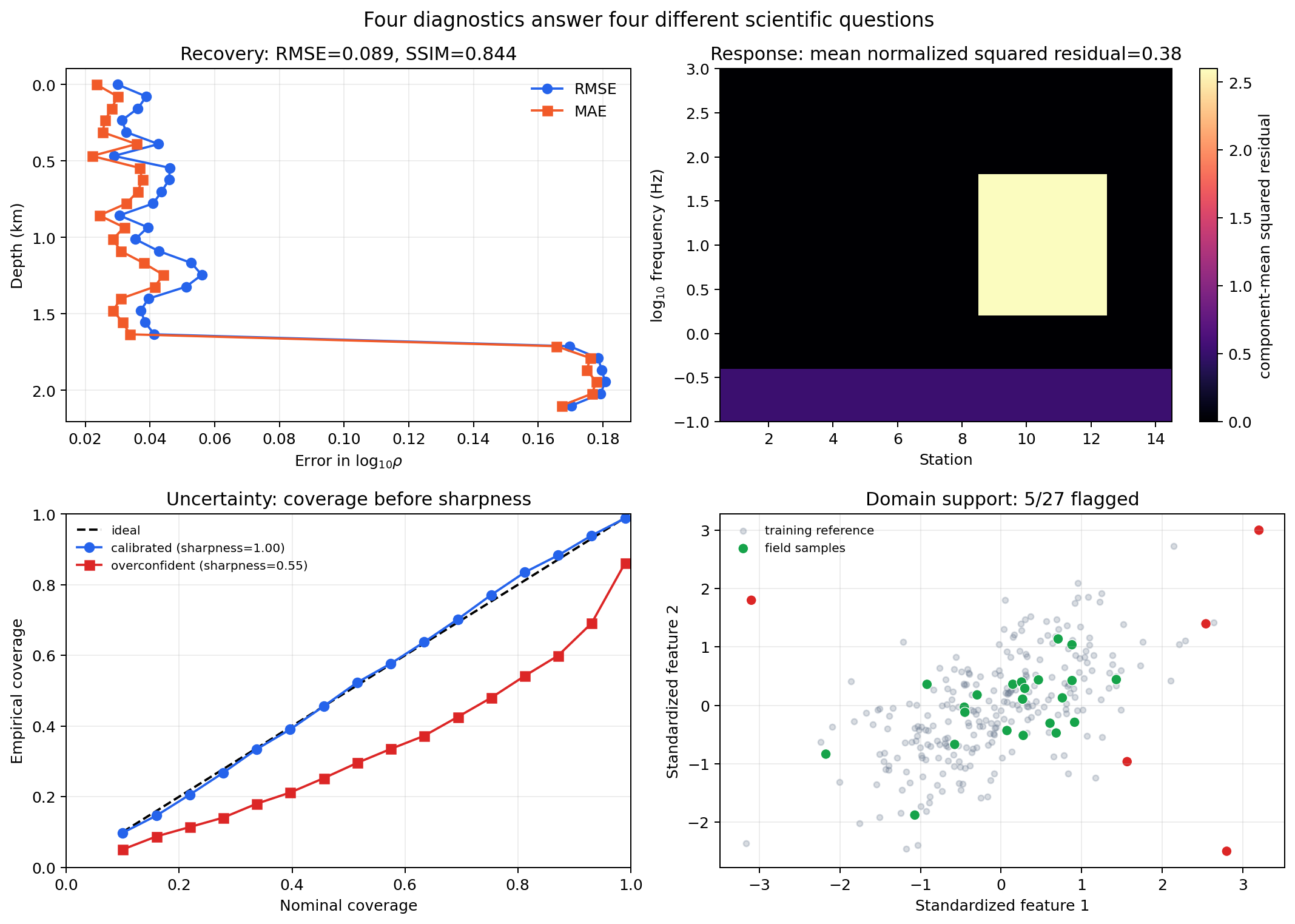
Four-panel executed validation audit showing depth recovery, station-frequency response residuals, uncertainty reliability, and out-of-distribution samples — Four reports generated from the current recovery, residual, calibration, and OOD APIs. Each panel retains the axis on which failure occurs.#

The recovery panel shows error increasing at depth even though the global RMSE remains below 0.09. The response heatmap localizes a component-specific misfit to stations 9–12 and a separate high-frequency edge effect; a global value of 0.375 would hide both structures. The reliability curves distinguish a correctly scaled predictor from a sharper but overconfident one. Finally, the domain panel retains five flagged samples rather than removing them before computing a reassuring average. Agreement in one panel cannot override a failure in another because model truth, response fit, uncertainty honesty, and deployment support are different validation claims.

6.3.16.7. Baselines and ablations#

AI inversion validation requires comparisons that answer whether the complexity adds value. Use the same held-out cases, preprocessing, units, and metrics for all methods. Relevant baseline model choices include:

a constant predictor based only on training-target medians;
a simple nearest-neighbour or low-capacity regression baseline;
the selected classical Occam, ModEM, or MARE2DEM workflow where dimensionality and data support permit;
an AI-initialized classical or hybrid refinement;
alternative AI architectures selected before test evaluation.

Compare accuracy, forward misfit, uncertainty calibration, runtime, memory, failure rate, and analyst effort. A model that is faster but less accurate may still be valuable as an initializer; state that narrower role rather than claiming replacement of classical inversion.

Because candidate and baseline are evaluated on the same held-out parents, compare them through paired differences. If \(E_{A,g}\) and \(E_{B,g}\) are errors for the AI model and baseline on independent parent survey \(g\), define improvement as

(4)#\[\Delta_g = E_{B,g}-E_{A,g}, \qquad \bar{\Delta}=\frac{1}{G}\sum_{g=1}^{G}\Delta_g.\]

Positive \(\Delta_g\) favors the AI model. Confidence limits for \(\bar{\Delta}\) must resample the independent parent surveys, not every correlated station window as though it were a new experiment.

The executed illustration contains 18 parent surveys with eight correlated rows each:

mean paired RMSE improvement: 0.0367
surveys favoring AI: 14 / 18
row-bootstrap 95% interval:    [0.0295, 0.0437]
survey-bootstrap 95% interval: [0.0173, 0.0561]

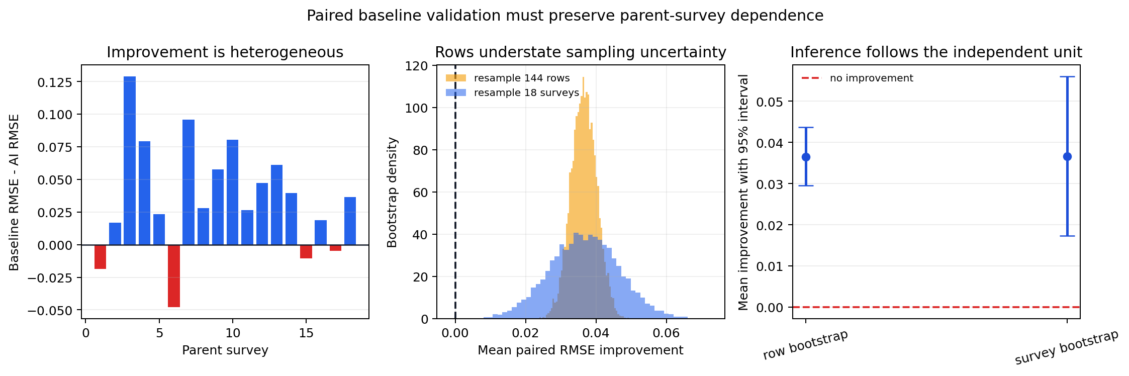
Per-survey paired improvements, row-level and survey-level bootstrap distributions, and their 95 percent intervals — The point estimate is unchanged, but uncertainty expands when resampling follows the actual independent unit.#

Four surveys favor the baseline, so the positive mean is not a universal-win claim. Treating 144 rows as independent produces a much tighter interval than resampling 18 surveys and overstates the precision of deployment-level improvement. The group interval remains positive in this controlled example, but the wider range is the defensible evidence. Stratify the paired deltas by geology, noise, dimensionality, and acquisition regime to learn where either method wins; do not select only the favorable strata after seeing the test result.

View and copy the parent-survey bootstrap auditClick to inspect and copy the complete code

def make_validation_paired_bootstrap() -> None:
    """Compare row and parent-survey bootstrap uncertainty for a baseline delta."""
    rng = np.random.default_rng(440)
    n_survey, rows_per_survey = 18, 8
    survey_effect = rng.normal(0.0, 0.055, n_survey)
    improvement = 0.035 + survey_effect
    row_delta = np.repeat(improvement, rows_per_survey)
    row_delta += rng.normal(0.0, 0.012, row_delta.size)
    survey_id = np.repeat(np.arange(n_survey), rows_per_survey)
    survey_delta = np.array([row_delta[survey_id == i].mean() for i in range(n_survey)])

    n_boot = 8000
    row_boot = row_delta[rng.integers(0, len(row_delta), (n_boot, len(row_delta)))].mean(1)
    group_boot = survey_delta[
        rng.integers(0, n_survey, (n_boot, n_survey))
    ].mean(1)
    row_ci = np.quantile(row_boot, [0.025, 0.975])
    group_ci = np.quantile(group_boot, [0.025, 0.975])

    fig, axes = plt.subplots(1, 3, figsize=(12.6, 4.2))
    axes[0].bar(np.arange(1, n_survey + 1), survey_delta,
                color=np.where(survey_delta >= 0, "#2563eb", "#dc2626"))
    axes[0].axhline(0, color="#111827", lw=1)
    axes[0].set(xlabel="Parent survey", ylabel="Baseline RMSE - AI RMSE",
                title="Improvement is heterogeneous")
    axes[0].grid(alpha=0.22, axis="y")

    axes[1].hist(row_boot, bins=55, density=True, alpha=0.62, color="#f59e0b",
                 label="resample 144 rows")
    axes[1].hist(group_boot, bins=55, density=True, alpha=0.55, color="#2563eb",
                 label="resample 18 surveys")
    axes[1].axvline(0, color="#111827", ls="--")
    axes[1].set(xlabel="Mean paired RMSE improvement", ylabel="Bootstrap density",
                title="Rows understate sampling uncertainty")
    axes[1].legend(frameon=False, fontsize=8)
    axes[1].grid(alpha=0.2)

    means = [row_boot.mean(), group_boot.mean()]
    lows = [row_ci[0], group_ci[0]]
    highs = [row_ci[1], group_ci[1]]
    axes[2].errorbar([0, 1], means,
                     yerr=[np.array(means) - lows, highs - np.array(means)],
                     fmt="o", color="#1d4ed8", capsize=6, lw=2)
    axes[2].axhline(0, color="#dc2626", ls="--", label="no improvement")
    axes[2].set_xticks([0, 1], ["row bootstrap", "survey bootstrap"], rotation=15)
    axes[2].set(ylabel="Mean improvement with 95% interval",
                title="Inference follows the independent unit")
    axes[2].legend(frameon=False, fontsize=8)
    axes[2].grid(alpha=0.22, axis="y")
    fig.suptitle("Paired baseline validation must preserve parent-survey dependence")
    fig.tight_layout()
    _save(fig, "validation_paired_bootstrap.png")
    print(
        "validation bootstrap:",
        {"mean": float(group_boot.mean()),
         "row_ci": np.round(row_ci, 4).tolist(),
         "survey_ci": np.round(group_ci, 4).tolist(),
         "surveys_improved": int(np.sum(survey_delta > 0)),
         "n_surveys": n_survey},
    )

Ablation study results determine which inputs and mechanisms matter. Repeat evaluation after removing phase, individual components, auxiliary modalities, graph edges, augmentation, or a physics-loss term. An unchanged score may reveal that a claimed information source is being ignored.

6.3.16.8. Robustness and stress testing#

Construct challenge sets before field deployment. Vary one factor at a time and then test realistic combinations:

noise amplitude, outliers, and coherent cultural interference;
missing frequencies, shortened bandwidth, and irregular sampling;
static shift and residual distortion;
station spacing, profile length, and coordinate error;
resistivity and thickness near or beyond training bounds;
thin conductors, sharp contrasts, anisotropy, and 2-D/3-D structures;
component loss or modality dropout;
graph radius, connectivity, and isolated stations;
alternative forward-model or discretization settings.

Plot performance against stress severity. Define the operating envelope at the point where error, coverage, or failure rate crosses a predeclared limit. Stress tests are not expected to all pass; their purpose is to reveal when the model should abstain.

If \(s\) denotes an ordered stress level and gate \(q\) passes when \(G_q(s)=1\), the supported boundary is

(5)#\[s_{\max} = \sup\left\{s:\prod_{q\in\mathcal{Q}}G_q(s)=1\right\}.\]

Equation (5) uses the intersection of mandatory gates. Averaging them into one composite score would allow strong performance on an easy metric to compensate for a critical physical failure. The executed sweep below increases one declared severity variable and applies fixed teaching thresholds: recovery RMSE at most 0.10, normalized response loss at most 1.0, nominal-90% coverage at least 0.85, and OOD fraction at most 0.10.

first coverage failure severity: 0.625
first OOD-fraction failure severity: 0.750
first response-loss failure severity: 1.125
first recovery-RMSE failure severity: 1.375
joint operating boundary: below 0.625

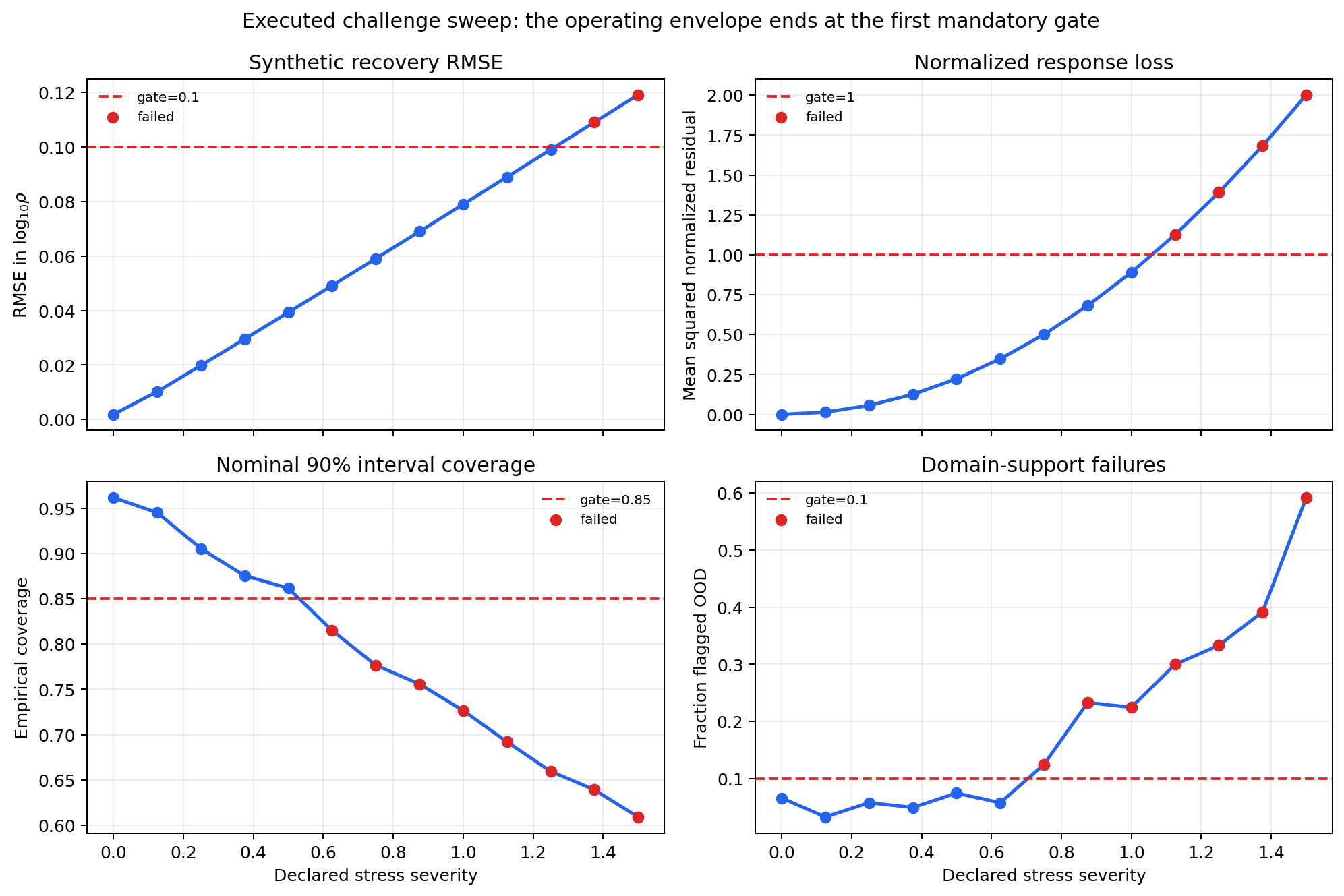
Four challenge-sweep curves showing recovery error, response residual, interval coverage, and OOD fraction crossing separate validation gates — A deterministic challenge sweep evaluated with the current recovery, response-residual, reliability, and OOD report functions.#

Parameter recovery is the last panel to fail, not the first. If this experiment reported only synthetic RMSE, it would claim support through severity 1.25; coverage has already failed at 0.625 and domain support at 0.75. The correct operating boundary therefore lies below 0.625. The ordering is itself useful: uncertainty becomes dishonest before the point estimate visibly collapses, then the input leaves reference support, followed by response and model-space failure. A real challenge axis should correspond to a physical quantity such as missing-frequency fraction, impedance noise, static-shift magnitude, or distance beyond the training resistivity range.

View and copy the executed operating-envelope sweepClick to inspect and copy the complete code

def make_validation_stress_envelope() -> None:
    """Execute all validation reports across one declared stress axis."""
    from scipy.ndimage import gaussian_filter

    rng = np.random.default_rng(1618)
    severity = np.linspace(0.0, 1.5, 13)
    nz, nx = 24, 36
    z = np.linspace(0, 1, nz)[:, None]
    x = np.linspace(-1, 1, nx)[None, :]
    truth = 2.4 + 0.45 * z - 1.0 * np.exp(
        -((x + 0.15) / 0.24) ** 2 - ((z - 0.52) / 0.17) ** 2
    )
    observed = np.ones((10, 18, 2), dtype=complex) * (60.0 + 35.0j)
    errors = np.full(observed.shape, 5.0)
    reference = rng.normal(size=(500, 4))

    recovery_rmse, response_loss, coverage, flagged = [], [], [], []
    for value in severity:
        prediction = gaussian_filter(truth, sigma=(0.35 + value, 0.5 + value))
        prediction = prediction + value * 0.13 * z
        recovery_rmse.append(recovery_report(prediction, truth).rmse)

        response_prediction = observed + value * (4.0 + 2.5j)
        report = response_residual_report(
            response_prediction, observed, errors=errors, kind="l2"
        )
        response_loss.append(report.overall.value)

        true_u = rng.normal(size=2400)
        mean_u = true_u + rng.normal(scale=0.25 + 0.24 * value, size=true_u.shape)
        std_u = np.full_like(true_u, 0.32)
        curve = reliability_curve(true_u, mean_u, std_u, levels=[0.90])
        coverage.append(curve.coverage[0])

        field = rng.normal(loc=value * 0.95, size=(120, 4))
        domain = flag_out_of_distribution(
            field, reference, method="mahalanobis", quantile=0.975
        )
        flagged.append(domain.fraction_flagged)

    recovery_rmse = np.asarray(recovery_rmse)
    response_loss = np.asarray(response_loss)
    coverage = np.asarray(coverage)
    flagged = np.asarray(flagged)
    thresholds = {"recovery": 0.10, "response": 1.0,
                  "coverage_low": 0.85, "ood_fraction": 0.10}

    fig, axes = plt.subplots(2, 2, figsize=(11.2, 7.5), sharex=True)
    panels = [
        (recovery_rmse, thresholds["recovery"], "Synthetic recovery RMSE",
         r"RMSE in $\log_{10}\rho$", False),
        (response_loss, thresholds["response"], "Normalized response loss",
         "Mean squared normalized residual", False),
        (coverage, thresholds["coverage_low"], "Nominal 90% interval coverage",
         "Empirical coverage", True),
        (flagged, thresholds["ood_fraction"], "Domain-support failures",
         "Fraction flagged OOD", False),
    ]
    for ax, (values, gate, title, ylabel, pass_above) in zip(axes.flat, panels):
        ax.plot(severity, values, "o-", color="#2563eb", lw=2)
        ax.axhline(gate, color="#dc2626", ls="--", label=f"gate={gate:g}")
        failed = values < gate if pass_above else values > gate
        ax.scatter(severity[failed], values[failed], color="#dc2626", zorder=4,
                   label="failed")
        ax.set(title=title, ylabel=ylabel)
        ax.grid(alpha=0.22)
        ax.legend(frameon=False, fontsize=8)
    for ax in axes[-1]:
        ax.set_xlabel("Declared stress severity")
    fig.suptitle("Executed challenge sweep: the operating envelope ends at the first mandatory gate")
    fig.tight_layout()
    _save(fig, "validation_stress_envelope.png")

    first_failures = {}
    for name, values, gate, pass_above in [
        ("recovery", recovery_rmse, thresholds["recovery"], False),
        ("response", response_loss, thresholds["response"], False),
        ("coverage", coverage, thresholds["coverage_low"], True),
        ("ood", flagged, thresholds["ood_fraction"], False),
    ]:
        failed = values < gate if pass_above else values > gate
        first_failures[name] = (
            None if not np.any(failed) else float(severity[np.flatnonzero(failed)[0]])
        )
    print("validation stress first failures:", first_failures)

6.3.16.9. Uncertainty validation#

For an ensemble inversion, point accuracy and uncertainty quality are separate axes. On an untouched test set, examine:

empirical versus nominal conformal coverage;
interval width or sharpness;
coverage by layer, depth, geology, and noise regime;
whether larger predicted spread corresponds to larger actual error;
forward-response coverage after propagating parameter draws;
behavior on deliberately shifted challenge cases.

For interval estimates \([L_{ij}(\alpha), U_{ij}(\alpha)]\) designed to cover target entry \(y_{ij}\) at nominal probability \(1-\alpha\), the entry-wise empirical coverage is

(6)#\[\widehat{C}(\alpha) = \frac{1}{|\mathcal{M}|} \sum_{(i,j)\in\mathcal{M}} \mathbf{1}\{L_{ij}(\alpha)\le y_{ij}\le U_{ij}(\alpha)\}.\]

Equation (6) measures entry-wise coverage. The mean interval width, \(|\mathcal{M}|^{-1}\sum_{(i,j)\in\mathcal{M}} \left(U_{ij}(\alpha)-L_{ij}(\alpha)\right)\), must be reported beside coverage, because overly wide intervals can cover well while still being scientifically unhelpful.

>>> import numpy as np
>>>
>>> y_test = np.array([
...     [2.0, 2.5, 3.0],
...     [2.1, 2.6, 2.9],
... ])
>>> lower = np.array([
...     [1.85, 2.35, 2.85],
...     [1.95, 2.45, 2.75],
... ])
>>> upper = np.array([
...     [2.15, 2.65, 3.15],
...     [2.25, 2.75, 3.05],
... ])
>>> alpha = 0.10
>>> entry_coverage = float(np.mean((lower <= y_test) & (y_test <= upper)))
>>> sample_coverage = float(np.mean(np.all(
...     (lower <= y_test) & (y_test <= upper), axis=1
... )))
>>> mean_width = np.mean(upper - lower, axis=0)
>>> print("nominal coverage:", 1.0 - alpha)
nominal coverage: 0.9
>>> print("entry coverage:", entry_coverage)
entry coverage: 1.0
>>> print("simultaneous sample coverage:", sample_coverage)
simultaneous sample coverage: 1.0
>>> print("mean 90% interval width:", np.round(mean_width, 3))
mean 90% interval width: [0.3 0.3 0.3]

Coverage measured on individual entries with ensemble.coverage is not the same diagnostic as the conformal simultaneous sample coverage. Label the definition used. See AI inversion uncertainty for the exchangeability assumptions and calibration set requirements.

6.3.16.10. Field-data validation#

Synthetic truth enables parameter scoring; field data rarely provide complete truth. Field validation therefore combines several weaker but independent lines of evidence:

Data compatibility: Confirm component order, units, phase convention, frequency support, missing-value handling, station geometry, and preprocessing match the validated feature contract.
Quality control: Review impedance validity, uncertainty, coherence or quality indicators, outliers, static shift, phase tensor, dimensionality, and strike. Load EDI data through pycsamt.emtools._core.ensure_sites(); do not bypass the canonical data model with ad-hoc arrays unless their provenance is retained.
Distribution support: Compare field feature ranges and distances with training and calibration distributions. Flag domain gap and out-of-distribution diagnostic results rather than interpreting a narrow ensemble spread as safety.
Forward consistency: Forward-model predicted structures and compare with the measured response and observational errors.
Method agreement: Compare with an appropriate classical inversion and with alternative parameterizations. Investigate disagreements instead of averaging them away.
External evidence: Compare interfaces and conductors with boreholes, logs, geology, hydrochemical information, seismic constraints, or known structures that were not used to tune the model.
Spatial coherence: Adjacent stations should vary in geologically plausible ways, but do not use smoothness alone as proof: a biased model can be smoothly wrong.

Blind wells or withheld geotechnical observations provide especially valuable checks. Keep them hidden until the workflow and interpretation rules are frozen.

6.3.16.11. Validation by inversion family#

1-D models: Validate resistivity, thickness, cumulative interface depth, response misfit, and lateral consistency across independently inverted stations. Diagnose where the 1-D assumption fails.
2-D U-Net models: Split at profile or parent-model level. Validate depth/lateral geometry, station-boundary effects, resizing behavior, and profile forward responses.
GCN models: Split at survey level. Verify node order and adjacency, then stratify error by node degree, edge distance, boundary location, and connected component. Compare against the identity-graph ablation.
Joint models: Validate row alignment and each modality independently. Test missing, corrupted, and shuffled modalities and compare against the strongest single-modality baseline.
PINN and hybrid models: Validate total and component losses, initial-model sensitivity, physics residual, observed-data misfit, regularization sensitivity, and convergence from multiple seeds. See Hybrid AI and physics inversion and Physics-informed 2-D inversion.

6.3.16.12. Failure analysis#

Do not report only representative successes. Create a failure table with one row per failed or high-error case and include:

case and parent-group identifier;
input quality and out-of-distribution indicators;
true and predicted parameter summaries where truth exists;
response residuals by frequency and component;
uncertainty interval and whether it covered the truth;
architecture, seed, and preprocessing version;
likely failure category and supporting evidence;
disposition: accepted limitation, abstention rule, data correction, or model redevelopment.

Inspect the worst cases by a metric chosen before opening them. Avoid deleting difficult cases unless a reproducible data-quality rule, independent of model error, requires exclusion.

6.3.16.13. Worked rejection decision#

The small FCN executed in Training AI inversion models is useful for demonstrating how separate gates combine. Before examining the results, suppose this teaching exercise requires log-resistivity MAE no greater than 0.3 in every layer, thickness MAE no greater than 100 m at every interface, no more than 10% of a field row outside the synthetic P1–P99 envelope, and dimensionality evidence compatible with station-wise 1-D interpretation. These are illustrative smoke test limits, not universal geophysical thresholds.

>>> print("resistivity layers passing:", 1, "/ 5")
resistivity layers passing: 1 / 5
>>> print("interfaces passing:", 0, "/ 4")
interfaces passing: 0 / 4
>>> print("WILLY stations requiring domain review:", 28, "/ 28")
WILLY stations requiring domain review: 28 / 28
>>> print("WILLY 3-D diagnostic fraction:", 0.856)
WILLY 3-D diagnostic fraction: 0.856
>>> decision = "rejected"
>>> print("validation decision:", decision)
validation decision: rejected

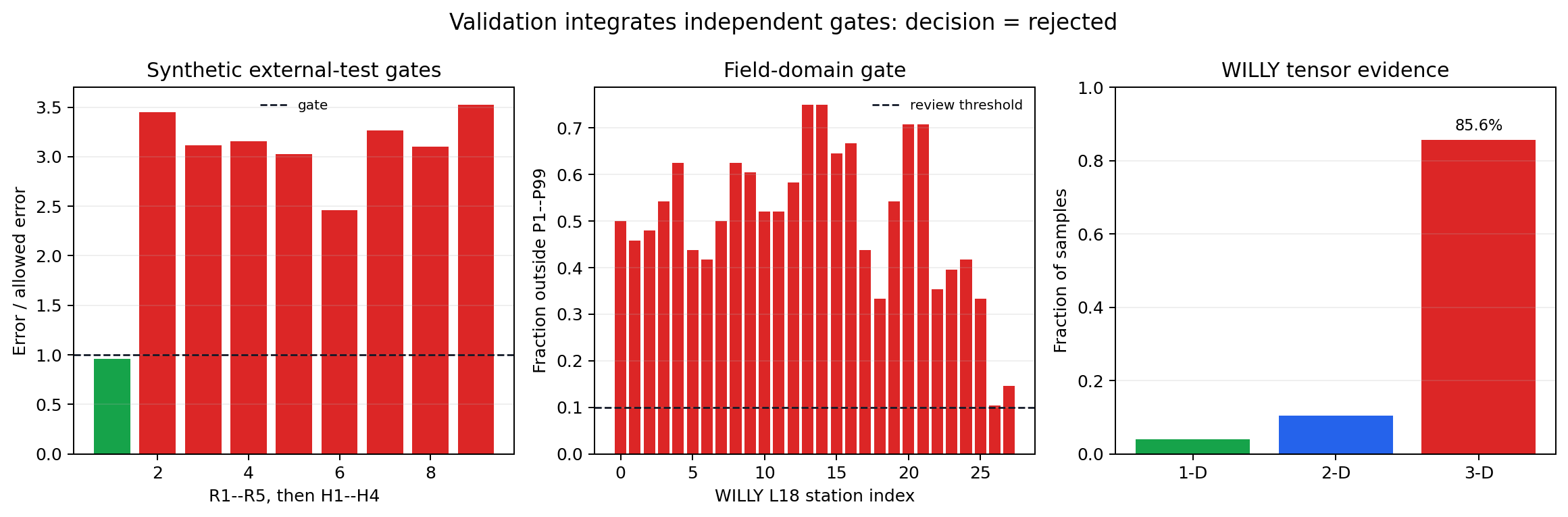
Validation dashboard combining synthetic errors, WILLY domain departure, and dimensionality evidence — Only the first resistivity layer passes the illustrative error limit, no interface passes, every WILLY station exceeds the marginal domain-review threshold, and most tensor samples classify as 3-D. Checkpoint restoration passed in the training audit, but that operational success cannot override four scientific failures.#

View and copy the executed rejection-dashboard codeClick to inspect and copy the complete code

def make_validation_gate_dashboard() -> None:
    frequency = np.logspace(np.log10(1.01), 4, 24)
    samples = generate_dataset(
        solver="mt1d",
        n_samples=240,
        freqs=frequency,
        n_layers=5,
        rho_range=(1.0, 10_000.0),
        depth_max=2000.0,
        noise_level=0.05,
        noise_type="field",
        include_phase=True,
        seed=137,
        n_jobs=1,
        output=None,
        verbose=False,
    )
    train, validation, test = samples.split(
        val_frac=0.15, test_frac=0.15, seed=137
    )
    pool_x = np.vstack([train.X, validation.X])
    pool_y = np.vstack([train.y, validation.y])
    inverter = EMInverter1D(
        n_features=48,
        n_layers=5,
        arch="fcn",
        solver="mt1d",
        device="cpu",
        log_thickness=False,
        augment_noise=0.01,
    )
    inverter.fit(
        pool_x,
        pool_y,
        epochs=25,
        batch_size=64,
        lr=1e-3,
        patience=7,
        val_frac=0.15,
        grad_clip=1.0,
        seed=137,
        verbose=False,
    )
    mae = np.mean(np.abs(inverter.predict(test.X) - test.y), axis=0)

    line = PROJECT_ROOT / "data" / "AMT" / "WILLY_data" / "L18PLT"
    sites = ensure_sites(line, recursive=True, verbose=0)
    field, _, station_names = sites_to_features_1d(
        sites, comp="xy", n_freqs=24, freq_min=1.01, freq_max=10_000.0
    )
    low, high = np.percentile(pool_x, [1, 99], axis=0)
    outside = np.mean((field < low) | (field > high), axis=1)
    dimension = classify_dimensionality(sites)["dim"].to_numpy(dtype=int)
    dim_fraction = np.array(
        [(dimension == value).mean() for value in (0, 1, 2)]
    )

    fig, axes = plt.subplots(1, 3, figsize=(13.0, 4.3))
    ax_error, ax_domain, ax_dim = axes
    normalized_error = np.r_[mae[:5] / 0.3, mae[5:] / 100.0]
    colors = [
        "#16a34a" if value <= 1 else "#dc2626" for value in normalized_error
    ]
    ax_error.bar(np.arange(1, 10), normalized_error, color=colors)
    ax_error.axhline(1.0, color="#111827", ls="--", lw=1.1, label="gate")
    ax_error.set(
        xlabel="R1--R5, then H1--H4",
        ylabel="Error / allowed error",
        title="Synthetic external-test gates",
    )
    ax_error.legend(frameon=False, fontsize=8)
    ax_error.grid(alpha=0.2, axis="y")

    station_index = np.arange(len(station_names))
    ax_domain.bar(station_index, outside, color="#dc2626")
    ax_domain.axhline(
        0.10, color="#111827", ls="--", lw=1.1, label="review threshold"
    )
    ax_domain.set(
        xlabel="WILLY L18 station index",
        ylabel="Fraction outside P1--P99",
        title="Field-domain gate",
    )
    ax_domain.legend(frameon=False, fontsize=8)
    ax_domain.grid(alpha=0.2, axis="y")

    ax_dim.bar(
        ["1-D", "2-D", "3-D"],
        dim_fraction,
        color=["#16a34a", "#2563eb", "#dc2626"],
    )
    ax_dim.set_ylim(0, 1)
    ax_dim.set(ylabel="Fraction of samples", title="WILLY tensor evidence")
    ax_dim.grid(alpha=0.2, axis="y")
    ax_dim.text(
        2,
        dim_fraction[2] + 0.025,
        f"{dim_fraction[2]:.1%}",
        ha="center",
        fontsize=9,
    )
    fig.suptitle(
        "Validation integrates independent gates: decision = rejected",
        fontsize=13,
    )
    fig.tight_layout()
    _save(fig, "validation_gate_dashboard.png")

The decision is rejection rather than conditional because failures occur inside the synthetic test problem as well as during field transfer. Response reconstruction was not supplied for this smoke checkpoint, so that mandatory gate is not evaluated, never silently counted as a pass. A production study would replace the illustrative thresholds, small dataset, and generic prior with predeclared project requirements and independent evidence.

6.3.16.14. Acceptance criteria#

Define thresholds from the intended scientific decision, observational error, baseline performance, and acceptable risk. Avoid universal thresholds such as “R-squared above 0.9” without context. A promotion gate can require all of the following:

parameter error below declared limits overall and in critical subgroups;
forward-response residual consistent with the data-error model;
improvement over the agreed baseline by a declared margin;
calibrated coverage close to nominal without excessive interval width;
no severe degradation inside the declared noise and acquisition envelope;
an out-of-distribution or QC rule that catches unsupported inputs;
acceptable failure, latency, and resource rates;
reproducible checkpoint reload and prediction;
documented review of worst cases and unresolved risks.

Use three outcomes rather than forcing pass or fail:

accepted: All mandatory gates pass for the stated intended use.
conditional: The model is allowed only inside a narrower operating envelope or with mandatory classical/analyst review.
rejected: Evidence is insufficient or a critical gate fails. Return to data design, model selection, or training rather than weakening the threshold after seeing results.

6.3.16.15. Statistical reporting#

Point estimates alone hide sampling variability. Report sample counts and confidence intervals for aggregate metrics, preferably using bootstrap units that respect the grouping structure. For example, resample whole geological realizations or surveys rather than correlated rows. Use paired resampling when comparing two methods on the same cases.

Report results across training seeds, but distinguish variation across seeds from uncertainty of the finite test sample. Do not select the best seed on the test set. If many architectures, groups, or metrics are inspected, acknowledge the resulting multiplicity and prioritize predeclared primary endpoints.

6.3.16.16. Minimum validation record#

The validation artifact should contain:

intended-use and exclusion statements;
immutable model, configuration, environment, and data identifiers;
partition manifest with grouping and leakage checks;
parameter metrics in model and physical units;
depth-, layer-, geology-, and quality-stratified results;
forward-response residual figures and tables;
baseline and ablation comparisons;
robustness, domain-shift, and uncertainty diagnostics;
field and independent-evidence comparisons;
complete failure analysis;
predeclared thresholds and final accepted, conditional, or rejected status.

6.3.16.17. Validation checklist#

Before signing off, confirm that:

no test or calibration case influenced training or model selection;
parent earths, profiles, and surveys do not cross partitions;
metrics use stated units, transforms, masks, and denominators;
physical geometry and forward responses were evaluated;
comparisons use identical held-out cases and preprocessing;
uncertainty coverage and width were both measured;
challenge tests define a credible operating envelope;
field inputs were checked for QC, dimensionality, and domain support;
failures and negative evidence remain visible;
the conclusion is limited to the tested intended use.

Validation is complete when another analyst can reproduce the evidence and reach the same promotion decision without relying on undocumented judgment. Carry that evidence into AI inversion reporting and, for field interpretation, the broader Interpretation workflow.