8.7. Export and reporting#

Interpretation reporting turns analysis into a reviewable and reproducible interpretation package. A useful report does more than display a polished resistivity section: it identifies the source data, processing and inversion decisions, interpretation assumptions, calibration evidence, uncertainty, limitations, and the exact products being delivered.

pyCSAMT provides focused exporters and plotting classes rather than a single make_report() function for interpretation. This separation is deliberate. CSV, XYZ, LAS, VTK, figures, configuration files, and narrative conclusions serve different audiences and must be assembled according to the project’s review and governance requirements. The report is therefore a translation layer between numerical products and review decisions: each quantity should keep its units, mathematical meaning, evidence class, and origin visible as it moves from code to table, figure, and narrative.

Reporting principle

A deliverable is not reproducible merely because it can be reopened. A reviewer must be able to identify its inputs, units, coordinate convention, method, assumptions, software version, uncertainty, and approval state.

8.7.1. Reporting objectives#

A complete interpretation package should allow another qualified reviewer to:

understand the survey and decision being supported;
trace every final product back to a reviewed inversion model;
distinguish measured, inverted, calibrated, and interpreted quantities;
reproduce the principal calculations and figures from the documented equations, inputs, and code paths;
inspect calibration residuals and withheld validation results;
identify unsupported areas and alternative explanations;
know which files are preliminary, superseded, approved, or authoritative;
reuse machine-readable outputs without guessing units or coordinates.

Those objectives are deliberately practical. A reviewer should be able to open the package months later and answer three questions without calling the author: what exactly was used, what exactly was computed, and what exactly is being claimed. The first question is answered by provenance and manifests, the second by equations, code paths, units, and exported tables, and the third by the narrative, figures, uncertainty statements, and approval record. When one of those links is missing, the report becomes a presentation artifact rather than a reproducible scientific record.

8.7.2. Recommended reporting workflow#

define the audience, decision, and approval level;
freeze the reviewed source model and interpretation configuration;
assign stable identifiers and output status;
generate machine-readable tables and grids;
generate figures using consistent scales and labels;
write the methods, results, uncertainty, and limitations narrative;
validate exported content independently of the in-memory objects;
assemble a provenance manifest and checksums;
complete scientific and technical review;
publish an immutable approved package while preserving working files.

8.7.3. 1. Define audience and reporting level#

Different audiences need different products:

Scientific reviewer: Requires data quality, inversion diagnostics, parameter rationale, calibration residuals, uncertainty, and alternative interpretations.
Project decision-maker: Requires the decision question, principal findings, confidence, risks, limitations, and recommended next actions in plain language.
GIS or modeling specialist: Requires coordinate reference, geometry, units, null handling, field definitions, and machine-readable files.
Field team: Requires station names, profile direction, target coordinates, depth reference, uncertainty, access constraints, and unambiguous maps.
Regulator or client: May require named standards, approval signatures, data lineage, controlled revisions, and explicit statements of professional responsibility.

Define the reporting level before export:

working: Internal exploratory output. It may change and must not be used for a final decision.
review: Frozen candidate package submitted for scientific or technical review.
approved: Versioned package that has passed the project’s acceptance procedure.
superseded: Previously issued package retained for audit but no longer authoritative.

Put the status in the report, manifest, and directory name—not only in an email or surrounding conversation.

Reporting level also controls tone. A working package may contain trial figures and unresolved questions, but it should be visibly provisional. A review package should be internally frozen: comments may still change it, but the files under review should not mutate silently. An approved package should read as a release, with stable identifiers, checksums, and a clear statement of responsibility. superseded does not mean “delete”; it means “retain, but do not use as the current authority.”

8.7.4. 2. Separate evidence classes#

Every table and figure should make clear which kind of quantity it contains:

Measured: Field or laboratory observations such as impedance, water level, EC, lithology, pumping-test transmissivity, or slug-test conductivity.
Processed: Corrected or derived observations such as filtered impedance, static-shift corrected responses, or QC metrics.
Inverted: Model properties estimated by fitting the geophysical observations, such as the calculated resistivity model (CRM).
Calibrated: A model modified or parameterized using borehole or field constraints, such as the calibrated new model (NM).
Interpreted: Geological or hydrogeological labels and derived properties based on assumptions and evidence.
Predicted: Values calculated at validation locations or under scenarios.

Do not combine these classes in one column named value without an origin field. A geological contact inferred from resistivity is not a measured borehole contact, even when they agree. This distinction matters because the same symbol can mean different things in the workflow. In the source model, pyCSAMT stores

\[m_{j,k} = \log_{10}\rho_{j,k},\]

where \(\rho_{j,k}\) is the cell resistivity in ohm metres at depth cell \(j\) and profile cell \(k\). Exports may write either \(m\) or the linear value \(\rho = 10^m\); the file name, field name, and manifest must say which representation was delivered.

The same discipline applies to interpretive labels. A lithology class assigned from resistivity is a conditional interpretation, \(\ell_{j,k}=g(\rho_{j,k}, C)\), where \(g\) is the configured classification rule and \(C\) represents context such as rock database, borehole constraints, hydrogeological setting, and calibration thresholds. Changing \(C\) can change \(\ell\) even when \(\rho\) is unchanged. That is why interpreted labels should carry method context instead of being reported as if they were direct observations.

8.7.5. 3. Freeze provenance before export#

Assign stable identifiers to the source survey, processing run, inversion run, interpretation run, and reporting package. A simple naming pattern is:

<project>_<line>_<stage>_<YYYYMMDD>_<revision>

For example:

willy_L18_interpretation_20260712_r01

Before generating final files, record:

project and survey-line identifiers;
input file inventory or upstream manifest;
processing and inversion run identifiers;
source-model method, RMS, mesh, and reliable depth range;
coordinate reference system, profile origin, azimuth, and vertical datum;
pyCSAMT and Python versions;
interpretation configuration and rock-database version;
boreholes and constraints used for calibration;
observations reserved for validation;
uncertainty bounds, sample count, seed, and failure rate;
author, reviewer, organization, timestamp, and status.

The source model and configuration should remain unchanged while the review package is generated. If either changes, issue a new interpretation run rather than silently replacing files inside the existing package.

Freezing provenance is less about bureaucracy than about preventing accidental branching. If a table is regenerated after a color scale, rock database, or water-table threshold changes, the table may still have the same name but no longer support the same conclusions. Treat the reviewed source model, configuration, and evidence inventory as an input vector,

\[\mathcal{I} = (M_\mathrm{src}, C_\mathrm{interp}, E_\mathrm{cal}, E_\mathrm{val}, S),\]

where \(M_\mathrm{src}\) is the source model, \(C_\mathrm{interp}\) is the interpretation configuration, \(E_\mathrm{cal}\) and \(E_\mathrm{val}\) are calibration and validation evidence, and \(S\) contains software and environment details. A different \(\mathcal{I}\) should produce a different run or revision identifier.

8.7.6. 4. Use a controlled directory structure#

A practical interpretation package can use:

willy_L18_interpretation_20260712_r01/
├── README.md
├── manifest.yml
├── CHANGELOG.md
├── source/
│   ├── inversion_manifest.yml
│   ├── model_snapshot.npz
│   └── residual_summary.csv
├── configuration/
│   ├── interpretation.yml
│   ├── petrophysics.yml
│   └── rock_database.csv
├── evidence/
│   ├── borehole_inventory.csv
│   ├── constraints.csv
│   └── validation_observations.csv
├── tables/
│   ├── stratigraphic_logs.csv
│   ├── hydro_cells.csv
│   ├── hydro_by_station.csv
│   ├── uncertainty_by_station.csv
│   └── validation_residuals.csv
├── grids/
│   └── calibrated_resistivity.vtk
├── logs/
│   └── S017.las
├── gis/
│   └── profile.xyz
├── figures/
│   ├── crm_nm_misfit.png
│   ├── hydraulic_K.png
│   └── uncertainty_profile.png
├── report/
│   └── technical_report.pdf
└── checksums.sha256

The exact structure may follow organizational standards. The important rule is to separate immutable sources, configuration, evidence, machine-readable outputs, visual products, and narrative reports.

This separation makes review failures easier to diagnose. If a figure looks wrong, the reviewer can ask whether the error comes from the source model, the interpretation configuration, the exported table, or only the plotting layer. Keeping those layers in separate folders also protects the package from a common late-stage problem: editing a graphic or spreadsheet by hand and losing the connection to the values that generated it.

8.7.7. 5. Export stratigraphic logs to CSV#

pycsamt.interp.export.to_csv() writes all pycsamt.interp.StratigraphicLog objects to a flat table:

from pathlib import Path
from pycsamt.interp import export

root = Path("willy_L18_interpretation_20260712_r01")
table_path = export.to_csv(
    logs,
    root / "tables" / "stratigraphic_logs.csv",
)
print(table_path)

Captured output from a two-station documentation fixture:

>>> print(table_path)
docs/_tmp/reporting_example/tables/stratigraphic_logs.csv

The output fields are:

station: Station identifier.
x_m: Along-profile position in metres.
depth_m: Depth below the model surface in metres.
rho_log10: \(\log_{10}\) resistivity where linear resistivity is in ohm metres.
rho_ohm_m: Linear resistivity in ohm metres.
lithology: Interpreted lithology label assigned to the depth cell.

The current exporter writes both resistivity columns. Its log_rho argument is retained in the signature, but does not remove either column. Consumers should select the explicitly named field rather than infer units from values.

The CSV is usually the most useful audit table because it is both readable and easy to compare in tests. Each row represents one station-depth cell, not a continuous geological interval. If a layer boundary falls between two model cell centers, the CSV will still report cell-centered values. For interval interpretation, state whether boundaries were inferred from cell centers, merged layers, borehole picks, or a separate interpolation rule.

Validate the CSV after writing:

import csv

with table_path.open(newline="", encoding="utf-8") as stream:
    reader = csv.DictReader(stream)
    required = {
        "station", "x_m", "depth_m",
        "rho_log10", "rho_ohm_m", "lithology",
    }
    missing = required.difference(reader.fieldnames or [])
    if missing:
        raise ValueError(f"Missing CSV fields: {sorted(missing)}")
    rows = list(reader)

if not rows:
    raise ValueError("The stratigraphic export is empty.")

For the same fixture, the first rows read back as:

>>> rows[:3]
[{'station': 'S001', 'x_m': '0.000', 'depth_m': '10.000', 'rho_log10': '1.54407', 'rho_ohm_m': '35.000', 'lithology': 'Aquifer'},
 {'station': 'S001', 'x_m': '0.000', 'depth_m': '30.000', 'rho_log10': '1.65321', 'rho_ohm_m': '45.000', 'lithology': 'Sand (wet)'},
 {'station': 'S001', 'x_m': '0.000', 'depth_m': '60.000', 'rho_log10': '2.20412', 'rho_ohm_m': '160.000', 'lithology': 'Basalt (weathered)'}]

Never use a spreadsheet’s automatic formatting as the authoritative copy. Station names may be converted to dates or numbers, and scientific notation or decimal separators can change across locales.

For reproducibility, a CSV table should also be checked numerically. The two resistivity columns should satisfy

\[\rho_{\Omega\mathrm{m}} \approx 10^{\rho_{\log_{10}}},\]

within the rounding precision written to the file. A mismatch usually means that a table was edited manually, read with the wrong delimiter or decimal locale, or regenerated from a different source model.

8.7.8. 6. Export Oasis Montaj XYZ#

pycsamt.interp.export.to_oasis_montaj_xyz() writes each station log as a / Line block:

import numpy as np

elevation_m = np.array([238.4, 239.1, 240.0, 239.6])

xyz_path = export.to_oasis_montaj_xyz(
    logs,
    root / "gis" / "profile.xyz",
    y=0.0,
    elevation=elevation_m,
    log_rho=False,
)

The beginning of a linear-resistivity XYZ file is:

/ pycsamt.interp - Oasis Montaj XYZ
/ Generated: 2026-07-19T05:59:43.919117
/ X  Y  Z  RESD  LITH
/ Line S001
         0.000         500.000       -10.000    35.00000  Aquifer
         0.000         500.000       -30.000    45.00000  Sand_(wet)
         0.000         500.000       -60.000   160.00000  Basalt_(weathered)

Coordinate behavior must be documented:

X is log.station_x, normally an along-profile distance, not necessarily an easting;
the y argument is one scalar assigned to every point;
without elevation, Z is negative depth;
with elevation, Z is surface elevation minus depth;
the elevation array must correspond to the log order;
log_rho=True writes log10 resistivity; False writes linear ohm-m resistivity;
spaces in lithology labels are converted to underscores.

This exporter does not attach a coordinate reference system or vertical datum. Include those in the manifest and, where possible, in a companion metadata file. Do not label profile distance as easting unless it has actually been converted into the project CRS.

With elevation supplied, the vertical coordinate is

\[Z_{j,k} = h_k - z_j,\]

where \(h_k\) is station elevation and \(z_j\) is positive-down model depth. Without elevation, \(h_k=0\) and the file contains negative depth. The sign convention should be repeated in the manifest because many GIS and modelling tools treat positive vertical coordinates as elevation.

Custom channel names can be supplied:

export.to_oasis_montaj_xyz(
    logs,
    root / "gis" / "profile_linear_rho.xyz",
    log_rho=False,
    channels=["PROFILE_X_M", "PROFILE_Y_M", "ELEV_M",
              "RHO_OHM_M", "LITHOLOGY"],
)

The custom header changes labels, not coordinate transformation or data semantics.

This point is important for GIS delivery. Renaming X to EASTING does not project the profile distance into a coordinate reference system. If the survey line has an origin \((E_0,N_0)\) and azimuth \(A\), a simple planar conversion from chainage \(s\) would be documented as

\[E = E_0 + s\sin A, \qquad N = N_0 + s\cos A,\]

with \(A\) measured clockwise from north. If that conversion has not been performed, the safer label is profile distance or chainage, not easting.

8.7.9. 7. Export individual LAS logs#

pycsamt.interp.export.to_las() writes one stratigraphic log as LAS 2.0:

las_path = export.to_las(
    logs[0],
    root / "logs" / "S017.las",
    well_name="S017",
    company="Example Hydrogeophysics Project",
    null_value=-9999.25,
    log_rho=False,
)

The header should be inspected before delivery. A minimal fixture begins:

~VERSION INFORMATION
 VERS.                  2.0:   CWLS log ASCII Standard - VERSION 2.0
 WRAP.                  NO:    ONE LINE PER DEPTH STEP
~WELL INFORMATION
 STRT.M          10.0000:  START DEPTH
 STOP.M          100.0000:  STOP DEPTH
 STEP.M          30.0000:  STEP
 NULL.           -9999.25:  NULL VALUE
 COMP.           pycsamt:  COMPANY

The depth curve is in metres. log_rho=True writes log10 resistivity; False writes linear resistivity. Review the LAS header and curves in the receiving application before delivery.

Warning

The current LAS exporter encodes lithology as hash(lithology) % 1000. Python hash randomization means these integer codes are not guaranteed to remain stable across processes. Do not treat them as a durable corporate lithology dictionary. Deliver an explicit station/depth/lithology CSV and a controlled code table when stable codes are required.

LAS output is a station-column interpretation, not a drilled well log unless the station actually represents a borehole and the interpretation has been validated accordingly. State EM-derived prominently in the report and curve description.

Depth sampling also deserves attention. LAS consumers often assume a regular depth step, but an EM model may have irregular depth centers or layer thicknesses. The current exporter writes the median depth increment as STEP. If exact intervals matter, deliver the CSV with explicit cell depths and lithology labels beside the LAS file, and state that the LAS is a curve exchange convenience rather than the authoritative stratigraphic interval table.

8.7.10. 8. Export calibrated models to VTK#

pycsamt.interp.export.to_vtk() writes a pycsamt.interp.ResistivityModel as an ASCII rectilinear grid:

vtk_path = export.to_vtk(
    calibrated_model,
    root / "grids" / "calibrated_resistivity.vtk",
    log_rho=False,
    field_name="rho_ohm_m",
)

The start of the exported grid records the rectilinear geometry:

# vtk DataFile Version 3.0
pycsamt.interp resistivity model
ASCII
DATASET RECTILINEAR_GRID
DIMENSIONS 2 4 1
X_COORDINATES 2 float
0.000 100.000
Y_COORDINATES 4 float
10.000 30.000 60.000 100.000
Z_COORDINATES 1 float

Important format details:

X coordinates are model x_centers;
model depths are written as the VTK Y coordinates;
the VTK Z dimension contains one coordinate at zero;
values are written as point data;
missing resistivity is written as -9999.0;
no CRS, vertical datum, topography, or interpretation confidence is embedded;
the function exports resistivity only, not porosity, saturation, K, or lithological labels.

Use field_name to encode units explicitly. A file named calibrated_model.vtk is still ambiguous unless the manifest states whether the field is CRM or NM, log10 or linear, and which depth and coordinate conventions apply.

VTK orientation is another common source of false disagreement. pyCSAMT writes the 2-D section as a rectilinear grid with profile coordinate on X and positive-down model depth on Y. Many 3-D viewers display Y as a horizontal or vertical-up coordinate unless the user changes the camera or axis labels. The manifest should therefore describe the intended section orientation, not only the file format. If a viewer requires elevation-positive-up display, create a derived visualization file and keep the original model-depth export unchanged.

8.7.11. 9. Export to Golden Software Surfer#

pycsamt.interp.export.to_surfer_grid() and pycsamt.interp.export.to_surfer_xyz() write a pycsamt.interp.ResistivityModel — or any other 2-D inversion result accepted by from_any() (Occam2D, ModEM, the backend-neutral InversionResult, an AI agent result, or a raw array) — for Golden Software Surfer:

grd_path = export.to_surfer_grid(
    calibrated_model,
    root / "grids" / "calibrated_resistivity.grd",
    log_rho=False,
    nx=2, ny=4,
)
xyz_path = export.to_surfer_xyz(
    calibrated_model,
    root / "grids" / "calibrated_resistivity.dat",
    log_rho=False,
)

to_surfer_grid writes Surfer’s DSAA regular-grid header first, then one row of Z-values per line, from ymin to ymax:

DSAA
4
100
-100 -10
3162.28
89 3162.28
441 1540.57
138 598.738
199.526

to_surfer_xyz writes the same model’s real cell centres directly, with no resampling:

X    Y       Z
000        -10.000 100.00000
000        -30.000 316.22777
000        -60.000 630.95734
000        -100.000        1584.89319
000      -10.000 199.52623
000      -30.000 398.10717
000      -60.000 1000.00000
000      -100.000        3162.27766

Important format details:

to_surfer_grid requires a regular grid — DSAA cannot represent an irregular one — so it resamples the model’s own x_centers/z_centers (log-depth Occam2D cells, mesh padding, …) onto a new uniform nx x ny grid first; to_surfer_xyz needs no such step and is exact;
Y is −depth by default (shallow near 0, deep negative), so the section reads shallow-up in Surfer’s own map view, matching to_oasis_montaj_xyz()’s convention;
pass elevation= (plus chainage= or the model’s own station_x) to either function to drape real terrain instead — Y becomes elevation − depth, exactly as the topography-draped tutorial figures do;
missing/masked cells are written as Surfer’s own blanking sentinel (1.70141e38) in to_surfer_grid, or simply omitted as rows in to_surfer_xyz — never as the literal text nan, which Surfer’s DSAA reader cannot parse;
a native Occam2D/ModEM result is not auto-cropped to the station-carrying core — pass model.clip_to_stations() first if Occam2D’s own wide boundary-padding columns should not appear in the grid.

As with VTK, no CRS, vertical datum, or interpretation confidence is embedded — state those in the manifest, not the filename.

8.7.12. 10. Export deterministic hydro results#

An pycsamt.interp.EMHydroResult provides two CSV levels:

hydro_result.to_csv(root / "tables" / "hydro_cells.csv")
hydro_result.station_report_csv(
    root / "tables" / "hydro_by_station.csv"
)

The cell-level file includes station, profile position, depth, log10 and linear resistivity, porosity, saturation, and hydraulic conductivity. The station summary includes water-table depth, saturated-zone porosity and K summaries, transmissivity, storativity, Dar–Zarrouk parameters, and the TDS indicator.

In the narrative, write these as derived quantities. For a station column with cell thickness \(\Delta z_j\), saturation \(S_j\), porosity \(\phi_j\), and hydraulic conductivity \(K_j\), the represented saturated thickness and transmissivity are commonly summarized as

\[b = \sum_{j \in \mathcal{S}} \Delta z_j, \qquad T = \sum_{j \in \mathcal{S}} K_j\,\Delta z_j,\]

where \(\mathcal{S}\) is the set of cells below the detected water table and inside the represented saturated interval. If a project excludes clay-rich or low-confidence cells from \(\mathcal{S}\), state that rule next to the table.

If saturated-zone summaries are weighted, document the weighting explicitly. For example, an arithmetic mean of hydraulic conductivity over saturated cells,

\[\bar{K} = \frac{1}{b}\sum_{j \in \mathcal{S}} K_j\,\Delta z_j,\]

answers a different question from a geometric mean of log-conductivity,

\[K_\mathrm{g} = 10^{\frac{1}{b}\sum_{j \in \mathcal{S}}\log_{10}(K_j)\Delta z_j}.\]

The arithmetic mean is dominated by high-conductivity cells and is natural for flow capacity. The geometric mean is less sensitive to isolated high values and is often more stable for heterogeneous media. A report should not use the word “average” without saying which mean was used.

Document these interpretation qualifications:

water table is threshold-derived and may be nan;
K is petrophysically derived, not measured;
transmissivity integrates the represented saturated model interval;
unconfined storativity is approximated from porosity;
TDS is based on configured scalar pore-water resistivity;
columns with failed water-table detection require special review, as explained in Hydrogeophysical interpretation.

If pandas is installed, hydro_result.to_dataframe() supports further review, but any derived table should retain the original field names and units.

8.7.13. 11. Export qualitative hydro interpretation#

A pycsamt.interp.HydroGeophysicalModel can write cell classifications and interpreted zones:

qualitative_model.to_csv(
    root / "tables" / "hydro_units.csv"
)
qualitative_model.zones_to_csv(
    root / "tables" / "aquifer_zones.csv"
)

The cell table contains hydro-unit labels and confidence values. The zone table contains station, position, top, bottom, thickness, mean resistivity, confidence, and zone type.

Report the rule set, thresholds, context, rock database, and evidence used to produce these categories. A numerical confidence emitted by a rule-based classifier is not automatically a calibrated probability.

Confidence values are best treated as internal support scores unless they have been calibrated against independent observations. A rule may assign high confidence because a resistivity value sits well inside a configured range, but that does not prove the geological unit is correct. Report the physical rule, the evidence that supports it, and the alternative units that could produce a similar response. In clay-rich aquifers, weathered basement, saline water, and conductive alteration can overlap in resistivity space, so context is part of the interpretation method rather than a footnote.

8.7.14. 12. Export uncertainty summaries#

pycsamt.interp.UncertaintyResult writes a per-station summary:

uncertainty.to_csv(
    root / "tables" / "uncertainty_by_station.csv"
)

The table includes water-table mean, standard deviation, P10, P90, P90–P10 range, detection percentage, and transmissivity summaries. Preserve the corresponding bounds, distribution type, free parameter order, sample count, seed, and failure diagnostics in configuration or manifest files.

For a Monte Carlo ensemble \(\{w_i\}_{i=1}^{N}\) of detected water-table depths, the mean and spread are

\[\bar{w} = \frac{1}{N_d}\sum_{i \in D} w_i, \qquad s_w = \sqrt{\frac{1}{N_d-1}\sum_{i \in D}(w_i-\bar{w})^2},\]

where \(D\) is the set of successful detections and \(N_d=|D|\). Percentiles such as P10 and P90 are empirical quantiles of the same successful set, while the detection percentage is \(100N_d/N\). This is why the failure count belongs in the uncertainty result rather than only in plotting notes.

The raw water-table and transmissivity ensembles returned by MonteCarloHydro.run_ensemble() are not written by this CSV method. Archive them separately in an appropriate binary array format when empirical probabilities or distribution plots must be reproduced.

State that the intervals are conditional on the sampled parameters and fixed source resistivity model. See Uncertainty and validation for uncertainty sources that remain outside this ensemble.

Use interval language carefully. A P10-P90 interval from the ensemble means that 80 percent of the accepted simulated outcomes fall between those two quantiles under the stated sampling assumptions. It is not the full possible range, and it is not automatically a regulatory confidence interval. If the source inversion model, structural interpretation, or borehole control is held fixed, the interval does not include errors from those sources. Good reports say both what varied and what was held fixed.

8.7.15. 13. Report calibration residuals#

When quantitative field constraints are used, retain per-constraint residuals:

residuals = calibrator.constraint_residuals(calibrated_result)

The method returns dictionaries rather than writing a file. Save them using a transparent table writer:

import csv

residual_path = root / "tables" / "calibration_residuals.csv"
residual_path.parent.mkdir(parents=True, exist_ok=True)

if residuals:
    fields = sorted({key for row in residuals for key in row})
    with residual_path.open("w", newline="", encoding="utf-8") as stream:
        writer = csv.DictWriter(stream, fieldnames=fields)
        writer.writeheader()
        writer.writerows(residuals)

Report individual residuals, not only the optimizer’s total objective. Clearly separate calibration observations from withheld validation observations.

Residuals should keep their sign and unit. Writing a residual as

\[e_i = y_i^\mathrm{obs} - y_i^\mathrm{pred}\]

lets the reviewer see whether the calibrated model is systematically too deep, too shallow, too resistive, or too conductive at the evidence locations. A single absolute or squared objective can hide bias. When observations have different units or reliability, also report the normalized residual

\[\tilde{e}_i = \frac{e_i}{\sigma_i},\]

where \(\sigma_i\) is the assigned observation uncertainty. The value of \(\sigma_i\) is part of the scientific assumption and belongs in the calibration record.

8.7.16. 14. Generate review figures and diagnostics#

Interpretation figures are review evidence and communication products. They should not be treated as decoration after the tables are finished. A good figure answers a review question: what changed during calibration, where is the interpreted aquifer, how variable is the water-table estimate, or which petrophysical assumption controls the result. pyCSAMT’s plotting classes are therefore best organized by the decision they support.

The examples below were generated from a small synthetic profile so the page can show what each class produces even when project data are not available. Use the same pattern with reviewed project objects, and write the generated PNG files into the package’s figures/ directory.

from pycsamt.interp import plot as iplot

figures = root / "figures"
figures.mkdir(parents=True, exist_ok=True)

fig = iplot.PlotCalibratedModel(
    crm,
    calibrated_model,
    calibrator.misfit_map(),
    vmin_rho=1.0,
    vmax_rho=4.5,
).plot()
fig.savefig(figures / "crm_nm_misfit.png", dpi=300,
            bbox_inches="tight")

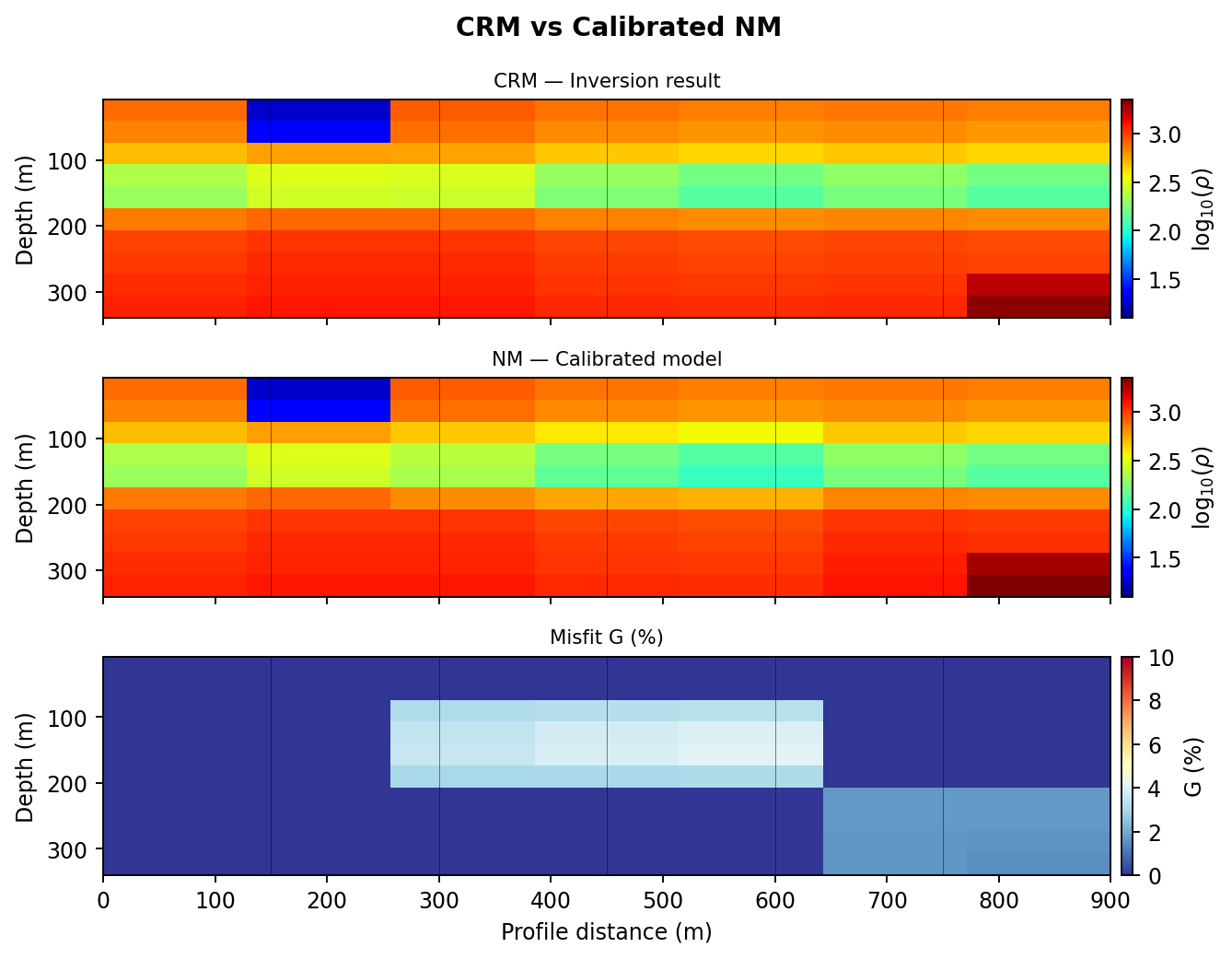
Calibrated model comparison showing CRM, NM, and misfit map. — `pycsamt.interp.plot.PlotCalibratedModel` compares the original calculated resistivity model, the calibrated new model, and the correction pattern. Use it whenever calibration changes are part of the evidence.#

Pseudo-stratigraphic figures translate cell values into station-scale interpretation. They are useful for reviewer checks because a reader can see both the interpreted layer pattern and the resistivity structure that supports it.

fig = iplot.PlotStratigraphicLog(logs[2]).plot()
fig.savefig(figures / "S03_stratigraphic_log.png", dpi=300,
            bbox_inches="tight")

fig = iplot.PlotFenceDiagram(
    logs,
    max_depth=260.0,
).plot()
fig.savefig(figures / "stratigraphic_fence.png", dpi=300,
            bbox_inches="tight")

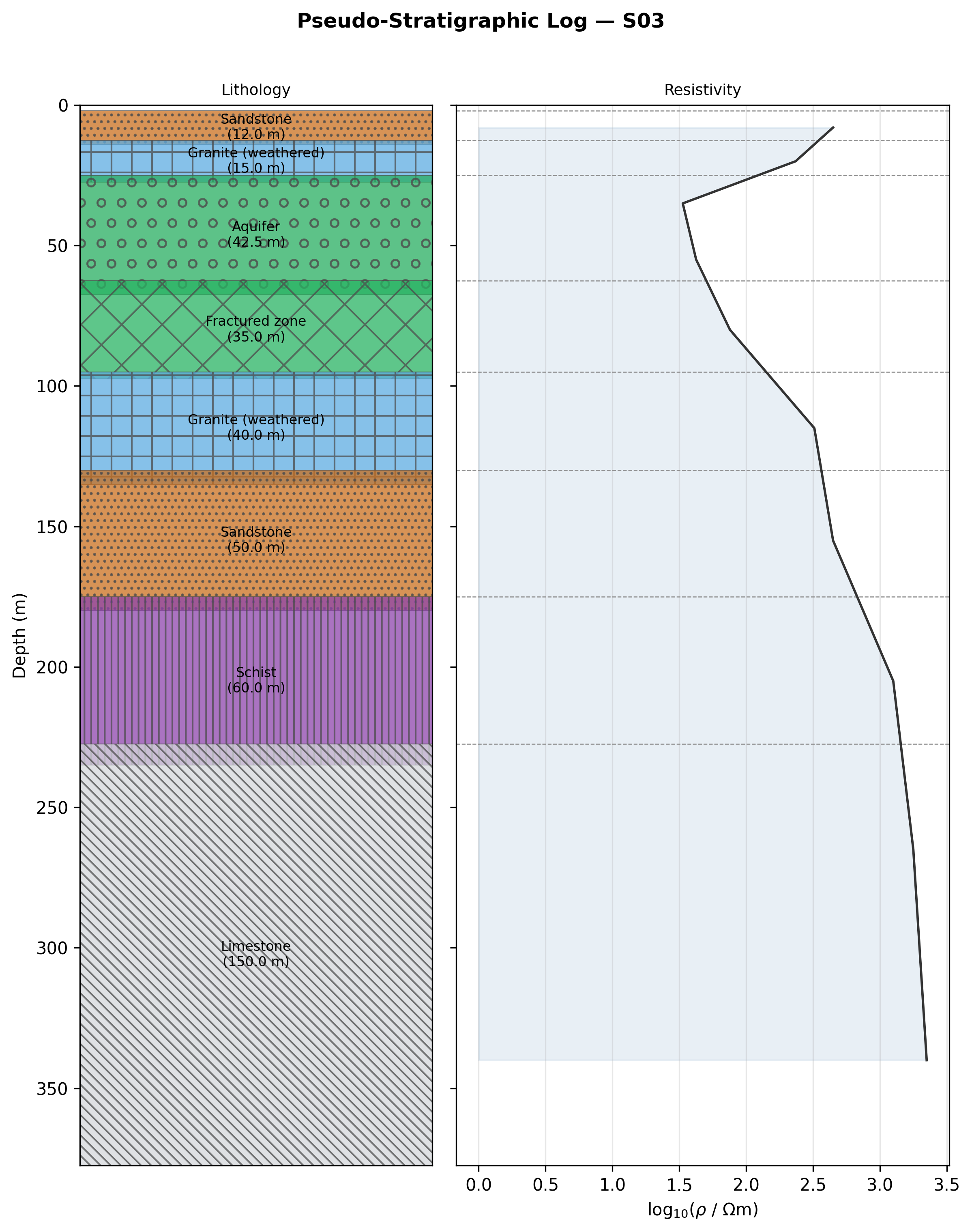
Single station pseudo-stratigraphic log with lithology and resistivity panels. — `pycsamt.interp.plot.PlotStratigraphicLog` is best for station-level review, especially when one borehole, target, or anomaly needs a detailed explanation.#

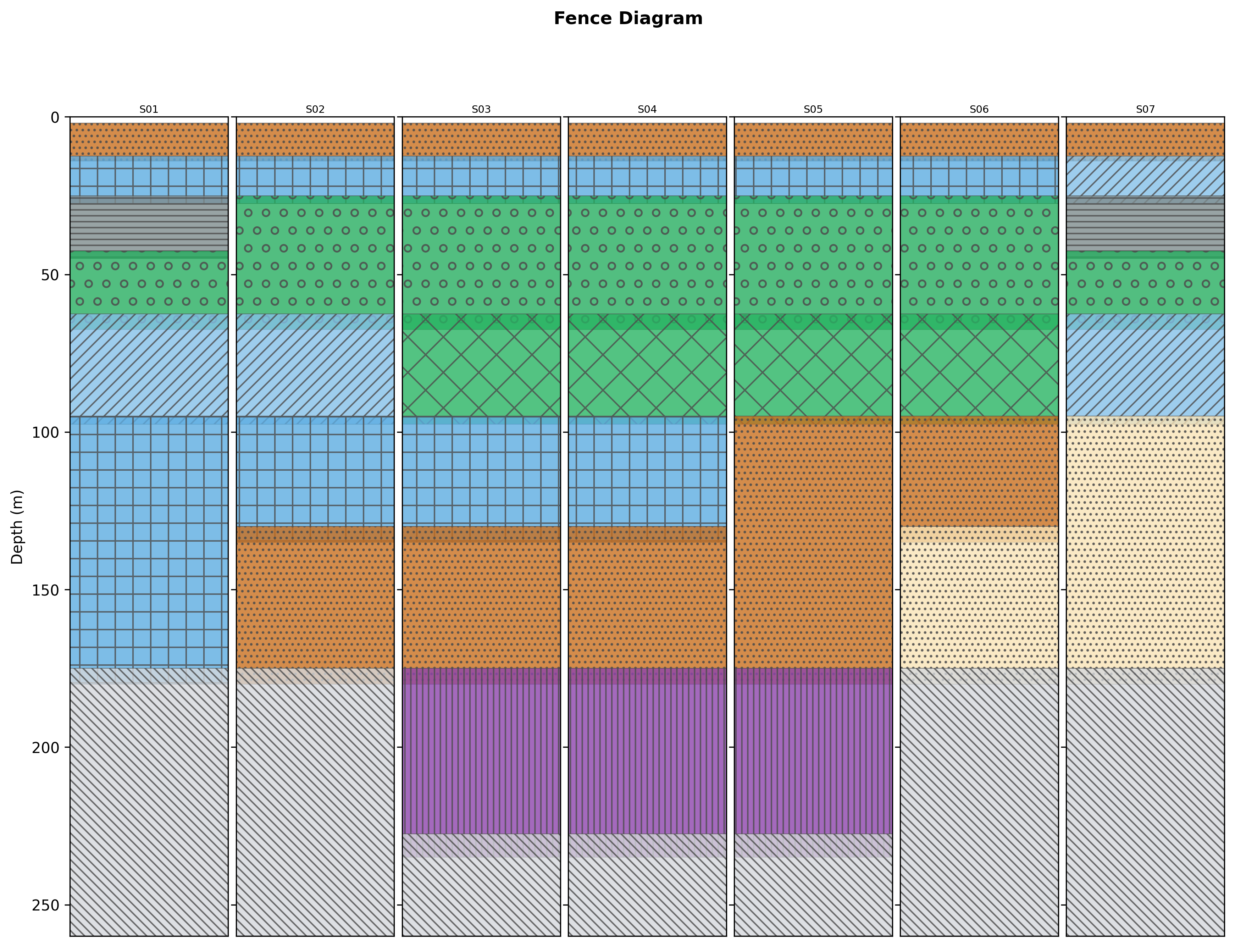
pycsamt.interp.plot.PlotFenceDiagram places station logs side by side so lateral changes can be inspected without treating the result as a fully interpolated geological section.#

Hydrogeophysical figures should make clear that the displayed quantities are derived from resistivity and petrophysical assumptions. They are most useful when paired with the equations and qualifications described earlier in this page.

fig = iplot.PlotHydroSection(
    hydro_result,
    quantity="K",
    vmin=-10.0,
    vmax=-3.0,
    depth_max=200.0,
).plot()
fig.savefig(figures / "hydraulic_K.png", dpi=300,
            bbox_inches="tight")

fig = iplot.PlotWaterTableProfile(
    hydro_result,
    reference_depth=70.0,
).plot()
fig.savefig(figures / "water_table_profile.png", dpi=300,
            bbox_inches="tight")

fig = iplot.PlotAquiferCharacterization(
    hydro_result,
    reference_depth=70.0,
).plot()
fig.savefig(figures / "aquifer_characterization.png", dpi=300,
            bbox_inches="tight")

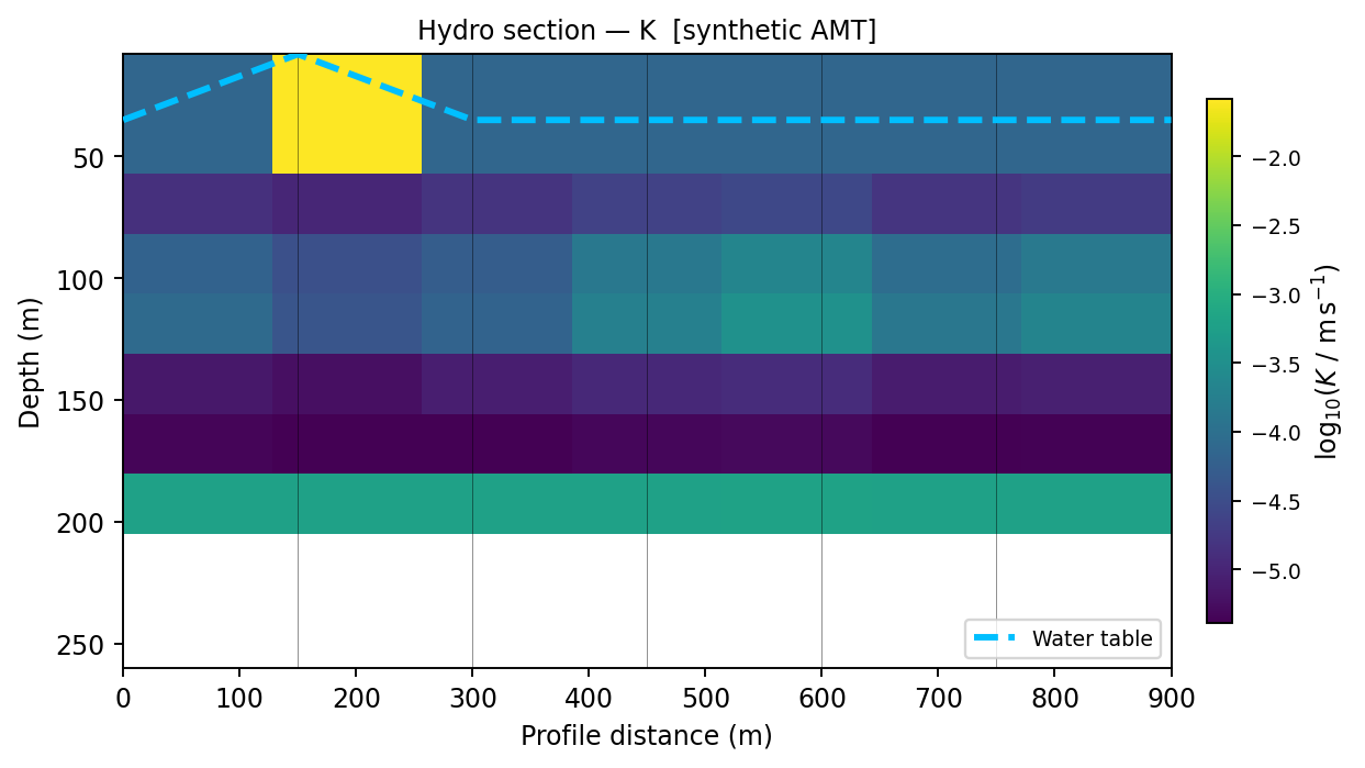
Hydrogeophysical section showing hydraulic conductivity and water table. — `pycsamt.interp.plot.PlotHydroSection` maps a cell-level hydro quantity such as `K`, saturation, or porosity over the model section. The caption should state the property, transform, and color limits.#

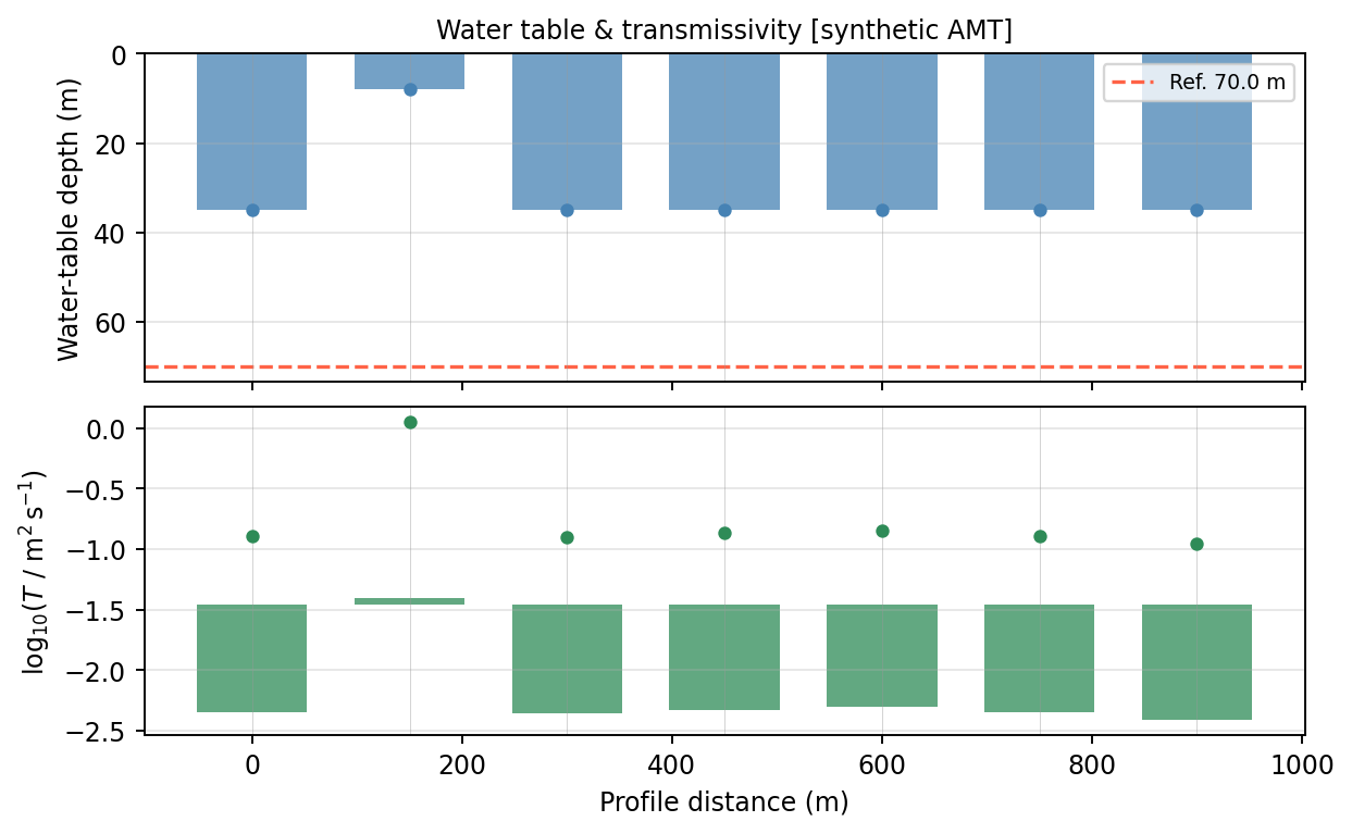
pycsamt.interp.plot.PlotWaterTableProfile summarizes station-level water-table depth and transmissivity. It is a compact way to show where hydro indicators strengthen, weaken, or fail along the line.#

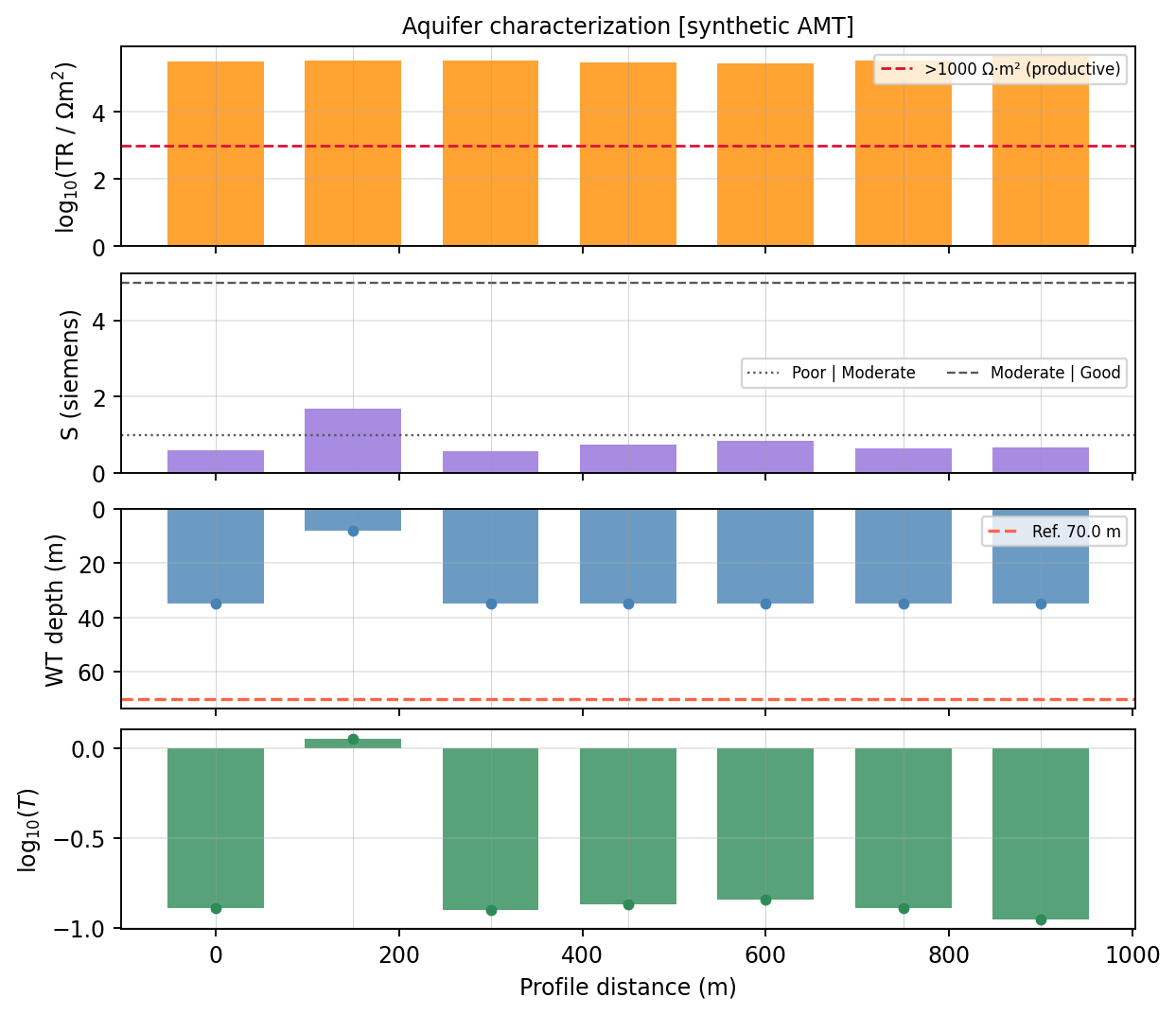
pycsamt.interp.plot.PlotAquiferCharacterization combines Dar-Zarrouk indicators, water table, and transmissivity. It is useful when reporting productivity and protective-capacity indicators together.#

Petrophysical diagnostics show whether the chosen transform is plausible for the cells being interpreted. They help separate a reporting claim from a hidden petrophysical assumption.

fig = iplot.PlotPetrophysicalCrossPlot(
    hydro_result,
    depth_range=(20.0, 260.0),
).plot()
fig.savefig(figures / "petrophysical_crossplot.png", dpi=300,
            bbox_inches="tight")

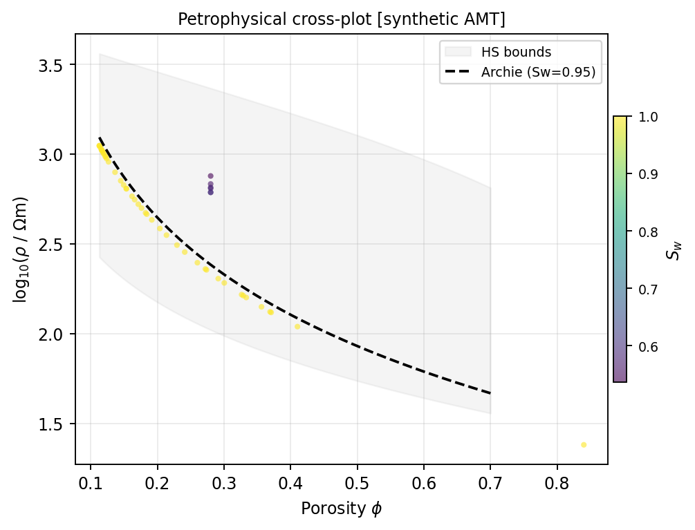
Petrophysical crossplot of porosity and resistivity colored by saturation. — `pycsamt.interp.plot.PlotPetrophysicalCrossPlot` compares cell porosity and resistivity against the selected petrophysical model. Use it to reveal whether the assumed Archie or Waxman-Smits relation is controlling a major conclusion.#

Uncertainty figures should be presented next to the deterministic figure they qualify. The goal is not only to show an interval, but to show where the interpretation is stable enough for the decision being made.

fig = iplot.PlotUncertaintySection(
    uncertainty,
    quantity="K",
    depth_max=200.0,
).plot()
fig.savefig(figures / "uncertainty_K_section.png", dpi=300,
            bbox_inches="tight")

fig = iplot.PlotUncertaintyProfile(
    uncertainty,
    reference_depth=70.0,
).plot()
fig.savefig(figures / "uncertainty_profile.png", dpi=300,
            bbox_inches="tight")

fig = iplot.PlotUncertaintyHistogram(
    uncertainty,
    quantity="water_table",
    stations=["S01", "S04", "S07"],
).plot()
fig.savefig(figures / "water_table_histograms.png", dpi=300,
            bbox_inches="tight")

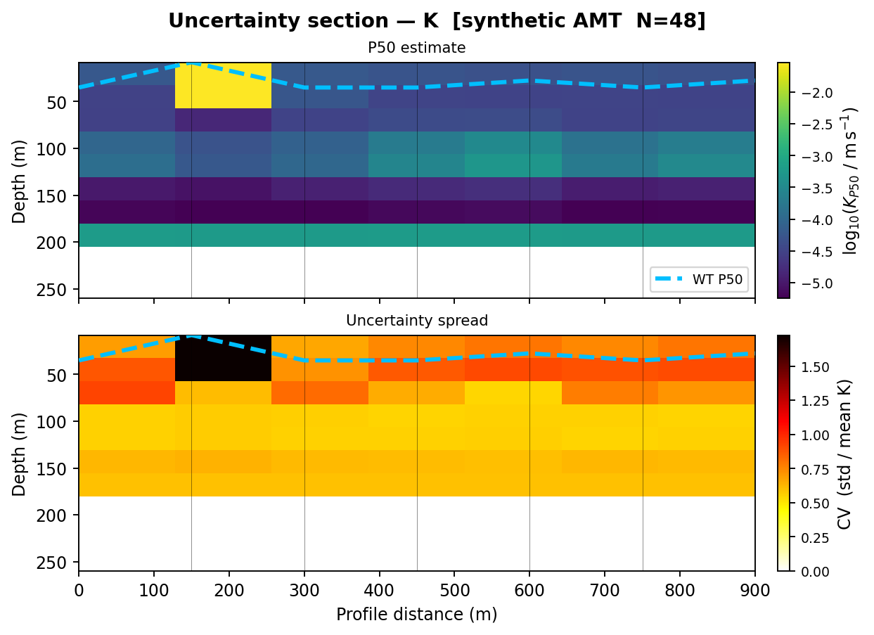
Uncertainty section with P50 hydraulic conductivity and spread. — `pycsamt.interp.plot.PlotUncertaintySection` shows the median estimate and spatial uncertainty spread on the same section geometry. This makes unsupported high-uncertainty zones visible instead of hiding them in a station table.#

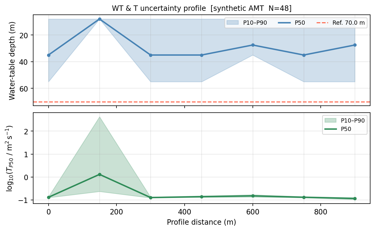
pycsamt.interp.plot.PlotUncertaintyProfile displays P10-P90 envelopes for water-table depth and transmissivity along the profile. It is the natural companion to pycsamt.interp.plot.PlotWaterTableProfile.#

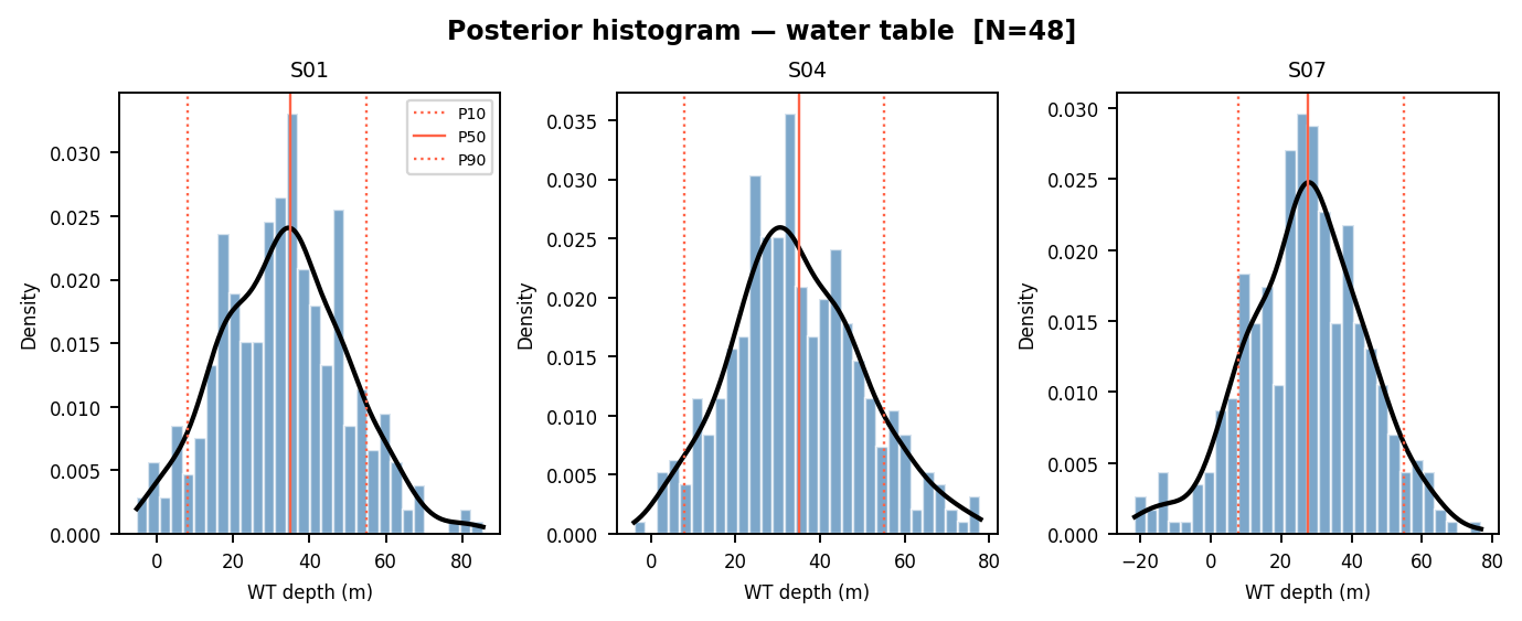
Water-table posterior histograms for selected stations. — `pycsamt.interp.plot.PlotUncertaintyHistogram` shows the posterior shape at selected stations. Use it when the interval is asymmetric, multi-modal, or otherwise poorly represented by a single P10-P90 band.#

A compact custom grid can still be helpful when a project needs side-by-side station-log figures that are not covered by a dedicated class. In that case, use Matplotlib axes directly and save the grid as a normal report figure:

A compact grid is often easier to compare than a stack of separate images. When several station-log figures are needed, create subplots with shared axes and save one review image:

>>> import matplotlib.pyplot as plt
>>> fig, axes = plt.subplots(1, 2, figsize=(7.2, 3.2), sharey=True)
>>> for ax, log in zip(axes, logs):
...     rho = 10.0 ** log.rho_log10
...     ax.step(rho, log.z_centers, where="mid")
...     ax.set_xscale("log")
...     ax.set_title(log.station_name)
...     ax.set_xlabel("rho (ohm m)")
...     ax.grid(True, which="both", alpha=0.3)
>>> axes[0].invert_yaxis()
>>> axes[0].set_ylabel("depth (m)")
>>> fig.tight_layout()
>>> fig.savefig(
...     "docs/source/images/user_guide/interpretation/"
...     "reporting_stratigraphic_logs.png",
...     dpi=180,
... )

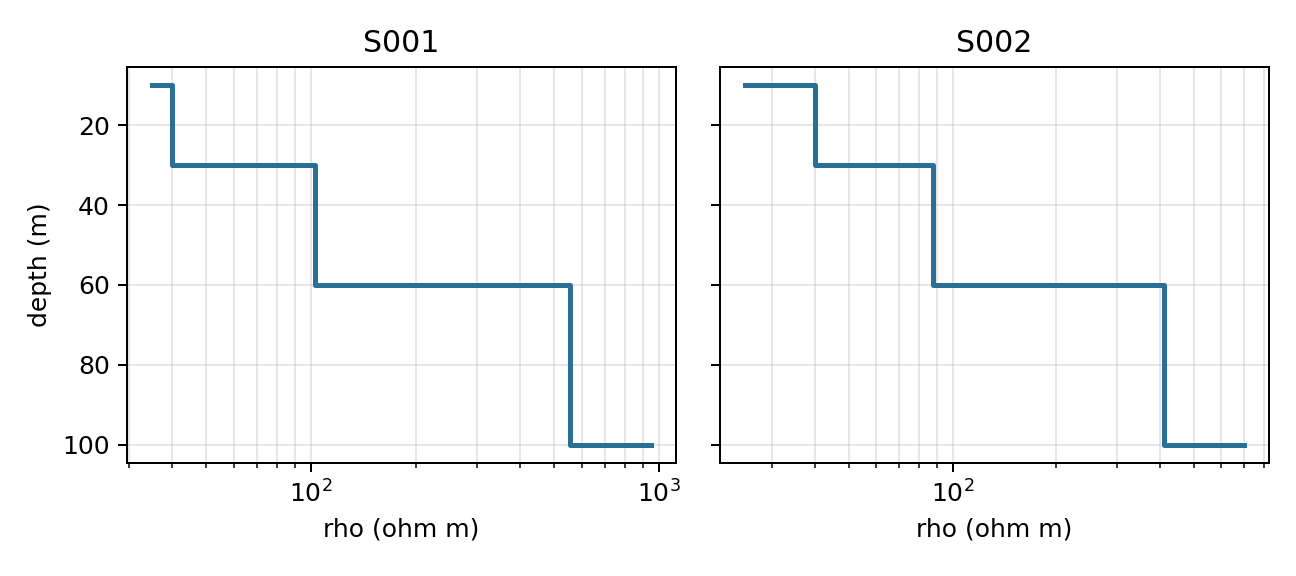
Two station resistivity-depth logs displayed in a shared-depth grid. — Captured output from the station-log plotting fixture. The shared depth axis makes the two columns comparable without repeating separate figures.#

8.7.16.1. Figure rules#

Every figure should identify:

project, line, method, and model status;
profile direction and horizontal coordinate;
depth or elevation reference and unit;
property and unit, including log transformation;
station locations where relevant;
consistent color scale across compared scenarios;
missing or masked cells;
water-table detection gaps;
uncertainty representation;
run or figure identifier.

Do not use different automatic color limits to compare scenarios. The same structure can appear stronger or weaker solely because the color normalization changed. Avoid rainbow palettes where they obscure ordering or accessibility, and check grayscale and color-vision readability when required by the project.

A figure should be reproducible from its caption and surrounding method text. For sections, state whether the vertical coordinate is depth below surface or elevation, whether the vertical exaggeration is one-to-one, and whether masked regions are outside the reliable depth of investigation or merely missing values. For comparison figures, record the normalization interval \([v_\min, v_\max]\), the colormap, and the transformation applied before plotting. For example, a hydraulic-conductivity section labelled log10(K m/s) and clipped to \([-10,-3]\) is not interchangeable with a linear K section in metres per second.

8.7.17. 15. Write the technical narrative#

A concise but complete interpretation report normally contains:

Executive summary: Decision, principal findings, confidence, limitations, and recommended next action. Avoid unexplained software or inversion terminology.
Objectives and scope: Survey area, question, target depth, methods, exclusions, and reporting status.
Data and processing: Acquisition inventory, data quality, exclusions, corrections, coordinate handling, and unresolved artifacts.
Inversion: Backend, dimensionality, mesh, errors, regularization, convergence, residuals, sensitivity, model scenarios, and reliable interpretation depth.
Interpretation method: CRM normalization, boreholes, rock database, calibration tolerance, classification logic, hydrogeophysical equations, and configuration.
Results: Observed patterns and derived quantities stated separately from geological hypotheses.
Calibration and validation: Evidence roles, residuals, withheld results, scale compatibility, matches, and mismatches.
Uncertainty: Data, inversion, petrophysical, calibration, and interpretive uncertainty; intervals and detection rates; assumptions not propagated.
Conclusions and recommendations: Answers to the stated questions, confidence-qualified targets, rejected alternatives, and specific follow-up measurements.
Limitations: Scientific, spatial, computational, and operational constraints that affect use of the deliverables.
Appendices: Configuration tables, file manifest, symbols and units, residuals, additional scenarios, and reviewer record.

The technical narrative should not repeat every exported row. Its job is to connect evidence to claims. A useful paragraph often follows the sequence observation -> method -> interpretation -> uncertainty -> implication. For example, describe the resistivity pattern first, then the calibration or hydrogeophysical rule used to interpret it, then the geological hypothesis, then the range of accepted alternatives, and only then the project implication. This keeps the reader from mistaking a compelling map color for a measured geological fact.

Keep observation and inference linguistically separate. For example:

observation: “A conductive zone occurs between profile distances 600 and 900 m below approximately 40 m depth.”;
interpretation: “The zone is consistent with saturated weathered material, but clay-rich material remains a plausible alternative.”;
validation: “BH03 intersects weathered granite in this interval; BH03 was withheld from calibration.”;
uncertainty: “The boundary varies from 35 to 58 m across accepted scenarios.”

Use the same discipline for negative findings. If a target is not supported, say whether the data lack sensitivity, the model is ambiguous, calibration contradicts the hypothesis, or uncertainty is too broad for the decision. “No aquifer detected” is a much stronger claim than “no supported aquifer interpretation within the reliable depth range.”

8.7.18. 16. Build a machine-readable manifest#

The manifest is the package’s index. YAML or JSON is suitable. A minimal YAML structure might be:

schema_version: 1
package_id: willy_L18_interpretation_20260712_r01
status: review
project: willy
survey_line: L18
created_utc: 2026-07-12T12:00:00Z
software:
  package: pycsamt
  version: 2.0.0
coordinates:
  horizontal_reference: profile_distance
  horizontal_unit: m
  vertical_reference: depth_below_surface
  vertical_positive: down
  vertical_unit: m
resistivity:
  linear_unit: ohm_m
  model_storage: log10_ohm_m
source_runs:
  processing: processing_run_id
  inversion: inversion_run_id
interpretation:
  run_id: interpretation_run_id
  calibration_boreholes: [BH01, BH02]
  validation_boreholes: [BH03]
uncertainty:
  n_samples: 500
  seed: 42
  interval: P10_P90
files:
  - path: tables/stratigraphic_logs.csv
    role: interpreted_station_cells
  - path: figures/crm_nm_misfit.png
    role: calibration_review

Extend this with checksums, sizes, media types, CRS identifiers, configuration hashes, and approval metadata according to project requirements. Do not put secrets, personal data, or machine-specific absolute paths in a deliverable manifest.

The manifest should be machine-readable but still understandable to a human reviewer. Prefer explicit field names such as vertical_positive: down over compressed local shorthand. For each file, include its role, units where relevant, producer step, and source dependency. A table that supports a conclusion should be traceable back to the model and configuration that made it; a figure should be traceable back to the table or model values it plotted. This turns the manifest into an audit map rather than a file listing.

8.7.19. 17. Add checksums and validate files#

Checksums detect accidental change after approval. Generate them with an organizationally approved tool and store paths relative to the package root. Checksums prove file integrity, not scientific correctness.

Validation should include:

Structural checks: Required files exist, are non-empty, and match manifest entries.
Schema checks: CSV headers, units, data types, null conventions, and unique identifiers are correct.
Numerical checks: Exported ranges and row counts agree with in-memory results; log and linear resistivity correspond; P10 ≤ P50 ≤ P90 where finite.
Coordinate checks: Profile distance, station order, elevation/depth convention, CRS, and datum agree across figures and files.
Visual checks: Figures open, labels are legible, color scales match comparisons, masked regions are visible, and no plotting layer was clipped.
Round-trip checks: Open each format in at least one target consumer when practical. Verify LAS curves, XYZ columns, VTK orientation, and CSV encoding.
Scientific checks: Conclusions match the approved tables and figures, calibration/validation roles are correct, and limitations are not omitted.

Validation should deliberately be independent of the code path that generated the file. Opening a CSV with the same object that wrote it proves little; it may reproduce the same mistake. Simple independent checks are often enough: count rows from the text file, recompute min/max values, verify that rho_ohm_m matches rho_log10, confirm that station names are unique where required, and open a few exported products in the target consumer. For scientific validation, compare claims against withheld observations before reviewing calibration successes, so the report does not accidentally reward overfitting.

8.7.20. 18. Review and approval#

Use separate review roles when project scale permits:

Scientific review: Tests geophysical, geological, hydrogeological, and uncertainty reasoning.
Technical review: Tests code paths, units, file schemas, reproducibility, and internal consistency.
Editorial review: Tests clarity, terminology, captions, accessibility, and audience fit.
Approval: Confirms that the package meets the project’s governance and release requirements.

Track comments and dispositions. If a review changes inputs, parameters, or conclusions, increment the revision and regenerate dependent outputs. Do not edit an approved binary or CSV in place.

8.7.21. 19. Handle revisions and superseded products#

Maintain a changelog with:

revision identifier and date;
author and approver;
files added, removed, or replaced;
scientific reason for change;
impact on conclusions and downstream users;
identifier of the superseded package.

Never reuse the same approved package identifier for different content. Preserve superseded packages in read-only archival storage with an obvious status marker. Notify downstream users when a revision changes target locations, depths, confidence, or safety-relevant conclusions.

8.7.22. 20. Protect sensitive information#

Interpretation packages can contain private well locations, infrastructure, landowner details, water-quality information, or commercially sensitive targets. Before release:

classify each file according to project policy;
remove unnecessary personal or machine-specific information;
limit coordinate precision when authorized and appropriate;
avoid embedding credentials, API keys, or local absolute paths;
verify image metadata and document properties;
separate public summaries from controlled technical appendices.

Do not reduce coordinate precision in a scientific archive unless the precise authoritative coordinates are preserved in an appropriately controlled source.

8.7.23. Complete export example#

The following example assembles core machine-readable products and figures. It assumes logs, crm, calibrated_model, calibrator, hydro_result, and uncertainty were created and reviewed as described in the preceding guides:

from pathlib import Path
import csv

from pycsamt.interp import export, plot as iplot

root = Path("willy_L18_interpretation_20260712_r01")
tables = root / "tables"
figures = root / "figures"
grids = root / "grids"
logs_dir = root / "logs"
gis = root / "gis"

for directory in (tables, figures, grids, logs_dir, gis):
    directory.mkdir(parents=True, exist_ok=True)

# Geological interpretation products.
export.to_csv(logs, tables / "stratigraphic_logs.csv")
export.to_oasis_montaj_xyz(
    logs, gis / "profile.xyz", log_rho=False
)
export.to_las(
    logs[0], logs_dir / f"{logs[0].station_name}.las",
    log_rho=False,
)
export.to_vtk(
    calibrated_model,
    grids / "calibrated_resistivity.vtk",
    log_rho=False,
    field_name="rho_ohm_m",
)

# Hydrogeophysical and uncertainty products.
hydro_result.to_csv(tables / "hydro_cells.csv")
hydro_result.station_report_csv(tables / "hydro_by_station.csv")
uncertainty.to_csv(tables / "uncertainty_by_station.csv")

# Calibration residuals.
residuals = calibrator.constraint_residuals(hydro_result)
if residuals:
    fields = sorted({key for row in residuals for key in row})
    with (tables / "calibration_residuals.csv").open(
        "w", newline="", encoding="utf-8"
    ) as stream:
        writer = csv.DictWriter(stream, fieldnames=fields)
        writer.writeheader()
        writer.writerows(residuals)

# Review figures with explicit comparison scales.
fig = iplot.PlotCalibratedModel(
    crm,
    calibrated_model,
    calibrator.misfit_map(),
    vmin_rho=1.0,
    vmax_rho=4.5,
).plot()
fig.savefig(figures / "crm_nm_misfit.png", dpi=300,
            bbox_inches="tight")

fig = iplot.PlotUncertaintyProfile(uncertainty).plot()
fig.savefig(figures / "uncertainty_profile.png", dpi=300,
            bbox_inches="tight")

This script creates files; it does not by itself create the narrative report, manifest, checksums, review record, or approval. Those are required parts of a controlled reporting workflow.

8.7.24. Delivery checklist#

Check	Acceptance evidence
Scope and status are explicit	Audience, decision, project, line, revision, and working/review/approved status.
Inputs are traceable	Survey, processing, inversion, interpretation, and configuration IDs.
Quantity classes are separated	Measured, inverted, calibrated, interpreted, and predicted fields are labeled.
Coordinates are unambiguous	CRS or profile reference, origin, direction, units, datum, and vertical sign convention.
Units are explicit	Linear/log resistivity, depth/elevation, K, T, storativity, EC, and TDS.
Exports are validated	Schema, row count, numerical range, null handling, target-application round trip, and manifest match.
Figures are comparable	Stable color limits, visible missing data, readable labels, and figure identifiers.
Calibration is reviewable	Constraints, fitted parameters, bounds, restarts, and residuals.
Validation is independent	Withheld evidence, prediction intervals, mismatches, and dispositions.
Uncertainty is conditional and complete	Bounds, samples, seed, failures, detection rates, scenarios, and omitted uncertainty sources.
Limitations and alternatives are stated	Reliable depth, resolution, conceptual ambiguity, and usage limits.
Package integrity is controlled	Manifest, checksums, changelog, reviewer, approver, and immutable copy.

8.7.25. Common reporting mistakes#

Avoid these errors:

delivering only a color image without source values or provenance;
labeling along-profile distance as easting;
mixing depth below surface with elevation above datum;
omitting whether resistivity is log10 or linear;
presenting calibrated lithology as directly observed geology;
treating LAS hash-based lithology codes as stable identifiers;
calling derived hydraulic conductivity a measured field value;
hiding water-table non-detections or Monte Carlo failures;
reporting P10–P90 as the complete range of possible outcomes;
changing color scales between scenarios;
using calibration wells again as independent validation;
manually editing exported tables without recording the change;
replacing an approved package without incrementing its revision;
assuming checksums establish scientific correctness;
omitting known alternative explanations because they complicate the summary.

8.7.26. Next steps#

Use this page with:

Interpretation workflow for geological interpretation and calibration;
Hydrogeophysical interpretation for deterministic hydrogeophysical products;
Uncertainty and validation for conditional intervals and validation;
Map Tools for spatial context and mapping exports;
Inversion for source-model provenance and diagnostics.