Dimensionality Assessment

pycsamt.emtools.dimensionality asks a practical question before interpretation or inversion: does each station-frequency sample behave like 1-D, 2-D, or 3-D electromagnetic structure?

The module provides two complementary routes:

• a rule-based classifier using phase-tensor skew and ellipticity;

• a sparse dictionary workflow that learns patterns from several impedance and phase-tensor features.

It also provides helper workflows for 2-D inversion preparation: masking 3-D samples, rotating data to strike, antisymmetrizing the off-diagonal impedance tensor, and writing a pre-2D assessment table.

Full callable signatures live in the API reference. This page focuses on workflow, outputs, interpretation, and concrete line-numbered examples.

Why Dimensionality Comes First

A 1-D inversion assumes horizontally layered structure. A 2-D inversion assumes a dominant strike direction and negligible variation along that strike. Real CSAMT/AMT data can violate both assumptions because of local conductors, galvanic distortion, 3-D bodies, station effects, or complex geology.

Dimensionality diagnostics do not replace inversion. They tell you how much caution to use before choosing an inversion strategy, period band, strike rotation, or masking rule.

Core Features

phase_features_table builds one row per station and frequency. The features combine phase-tensor quantities with determinant-style impedance quantities:

Column	Meaning
station	Station name.
freq	Frequency in hertz.
period	Period in seconds.
beta_abs	Absolute phase-tensor skew angle, in degrees.
ellipt_abs	Absolute phase-tensor ellipticity.
logrho_det	log10 determinant-style apparent resistivity.
phi_det	Determinant impedance phase, in degrees.
tip_amp	Tipper amplitude when tipper data are available; otherwise NaN.

The determinant-style apparent resistivity uses the same practical EDI unit convention used elsewhere in emtools:

\[\rho_{det} = \sqrt{ \left(0.2 {|Z_{xy}|^2 \over f}\right) \left(0.2 {|Z_{yx}|^2 \over f}\right) }\]

Rule-Based Labels

The default rule uses two thresholds:

skew_th = 3.0
ellipt_th = 0.2

The class labels are:

dim = 0  ->  1-D
dim = 1  ->  2-D
dim = 2  ->  3-D

The rule is intentionally simple:

if beta_abs <= skew_th and ellipt_abs <= ellipt_th:
    dim = 0
elif beta_abs <= skew_th and ellipt_abs > ellipt_th:
    dim = 1
else:
    dim = 2

In other words, high phase-tensor skew pushes a sample into the 3-D class. Low skew with low ellipticity is treated as 1-D. Low skew with higher ellipticity is treated as 2-D.

Build The Feature Table

Start with the raw feature table before interpreting any labels.

from pathlib import Path

from pycsamt.emtools.dimensionality import phase_features_table

edi_dir = Path("data/AMT/WILLY_DATA/L18PLT")

features = phase_features_table(
    edi_dir,
    recursive=True,
    on_dup="replace",
    strict=False,
    verbose=0,
)

cols = [
    "station",
    "freq",
    "period",
    "beta_abs",
    "ellipt_abs",
    "logrho_det",
    "phi_det",
    "tip_amp",
]
print(features[cols].head())

   station     freq    period  ...  logrho_det    phi_det  tip_amp
0  18-001A  10400.0  0.000096  ...    1.886481  63.023441      NaN
1  18-001A   8707.0  0.000115  ...    1.925638  61.655406      NaN
2  18-001A   7289.0  0.000137  ...    1.948138  59.889966      NaN
3  18-001A   6102.0  0.000164  ...    2.061820  58.836496      NaN
4  18-001A   5108.0  0.000196  ...    2.182395  51.323119      NaN

[5 rows x 8 columns]

Line 7 loads the EDI directory through the shared ensure_sites machinery. Lines 15-24 show the columns most often used in downstream checks.

Inspect One Station

A single-station view makes the thresholds tangible.

import matplotlib.pyplot as plt

from pycsamt.emtools.dimensionality import phase_features_table

skew_th = 3.0
ellipt_th = 0.2

features = phase_features_table("data/AMT/WILLY_DATA/L18PLT")
station = "18-001A"
one = features.loc[features["station"] == station].sort_values("period")

fig, (ax_beta, ax_ellipt) = plt.subplots(
    2,
    1,
    figsize=(7, 6),
    sharex=True,
)

ax_beta.semilogx(one["period"], one["beta_abs"], "o-")
ax_beta.axhline(skew_th, color="0.4", linestyle="--")
ax_beta.set_ylabel("|beta| (deg)")

ax_ellipt.semilogx(one["period"], one["ellipt_abs"], "o-", color="C3")
ax_ellipt.axhline(ellipt_th, color="0.4", linestyle="--")
ax_ellipt.set_xlabel("Period (s)")
ax_ellipt.set_ylabel("Ellipticity")

fig.suptitle(f"{station} dimensionality features")
fig.tight_layout()

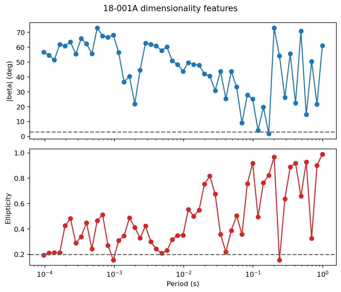
If beta_abs stays above the skew threshold over most periods, the station will be classified mostly 3-D regardless of ellipticity. If beta_abs is low, ellipticity separates 1-D from 2-D behavior.

Classify The Survey

Use classify_dimensionality to add the dim label to the feature table.

import pandas as pd

from pycsamt.emtools.dimensionality import classify_dimensionality

dim = classify_dimensionality(
    "data/AMT/WILLY_DATA/L18PLT",
    skew_th=3.0,
    ellipt_th=0.2,
)

counts = (
    dim.groupby("station")["dim"]
    .value_counts(normalize=True)
    .rename("fraction")
    .reset_index()
)

label = {0: "1D", 1: "2D", 2: "3D"}
counts["label"] = counts["dim"].map(label)
print(counts.head(12))

    station  dim  fraction label
0   18-001A    2  0.981132    3D
1   18-001A    1  0.018868    2D
2   18-002U    2  0.981132    3D
3   18-002U    1  0.018868    2D
4   18-003A    2  0.981132    3D
5   18-003A    1  0.018868    2D
6   18-004A    2  0.981132    3D
7   18-004A    1  0.018868    2D
8   18-005U    2  0.943396    3D
9   18-005U    1  0.056604    2D
10  18-006A    2  0.962264    3D
11  18-006A    1  0.037736    2D

Line 5 uses the default rule. Lines 11-15 compute station-level fractions so you can see whether a station is mostly 1-D/2-D or mostly 3-D.

Read The Rule In Feature Space

The clearest way to understand the rule is to plot beta_abs against ellipt_abs.

import matplotlib.pyplot as plt

from pycsamt.emtools.dimensionality import classify_dimensionality

skew_th = 3.0
ellipt_th = 0.2
dim = classify_dimensionality(
    "data/AMT/WILLY_DATA/L18PLT",
    skew_th=skew_th,
    ellipt_th=ellipt_th,
)

colors = {0: "tab:green", 1: "tab:blue", 2: "tab:red"}
labels = {0: "1-D", 1: "2-D", 2: "3-D"}

fig, ax = plt.subplots(figsize=(6.5, 5.5))
for cls in (2, 1, 0):
    sub = dim.loc[dim["dim"] == cls]
    ax.scatter(
        sub["beta_abs"],
        sub["ellipt_abs"],
        s=8,
        alpha=0.45,
        color=colors[cls],
        label=labels[cls],
    )

ax.axvline(skew_th, color="0.2", linestyle="--")
ax.axhline(ellipt_th, color="0.2", linestyle="--")
ax.set_xlabel("|beta| (deg)")
ax.set_ylabel("Ellipticity")
ax.legend()
fig.tight_layout()

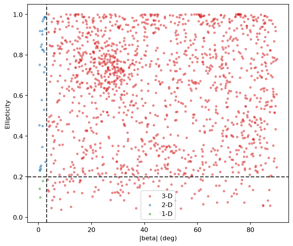
The vertical line is the 3-D boundary. The horizontal line separates 1-D and 2-D only on the low-skew side of the plot.

Threshold Sensitivity

Do not tune thresholds blindly. Sweep them and report how the dimensionality fractions change.

import numpy as np
import pandas as pd

from pycsamt.emtools.dimensionality import phase_features_table

features = phase_features_table("data/AMT/WILLY_DATA/L18PLT")

beta = features["beta_abs"].to_numpy()
ellipt = features["ellipt_abs"].to_numpy()
skew_thresholds = np.array([1, 2, 3, 5, 8, 12, 18, 25, 35, 50])
ellipt_th = 0.2

rows = []
for skew_th in skew_thresholds:
    low_skew = beta <= skew_th
    frac_1d = np.mean(low_skew & (ellipt <= ellipt_th))
    frac_2d = np.mean(low_skew & (ellipt > ellipt_th))
    frac_3d = 1.0 - frac_1d - frac_2d
    rows.append(
        {
            "skew_th": skew_th,
            "frac_1d": frac_1d,
            "frac_2d": frac_2d,
            "frac_3d": frac_3d,
        }
    )

sensitivity = pd.DataFrame(rows)
print(sensitivity)

   skew_th   frac_1d   frac_2d   frac_3d
0        1  0.001348  0.005391  0.993261
1        2  0.002022  0.012803  0.985175
2        3  0.002022  0.018868  0.979111
3        5  0.004717  0.028302  0.966981
4        8  0.008086  0.053235  0.938679
5       12  0.013477  0.079515  0.907008
6       18  0.018868  0.148922  0.832210
7       25  0.022237  0.249326  0.728437
8       35  0.033693  0.395553  0.570755
9       50  0.044474  0.537736  0.417790

If the 3-D fraction stays high over a wide threshold range, the result is probably a property of the data. If the fractions flip abruptly near one threshold, report that sensitivity with the interpretation.

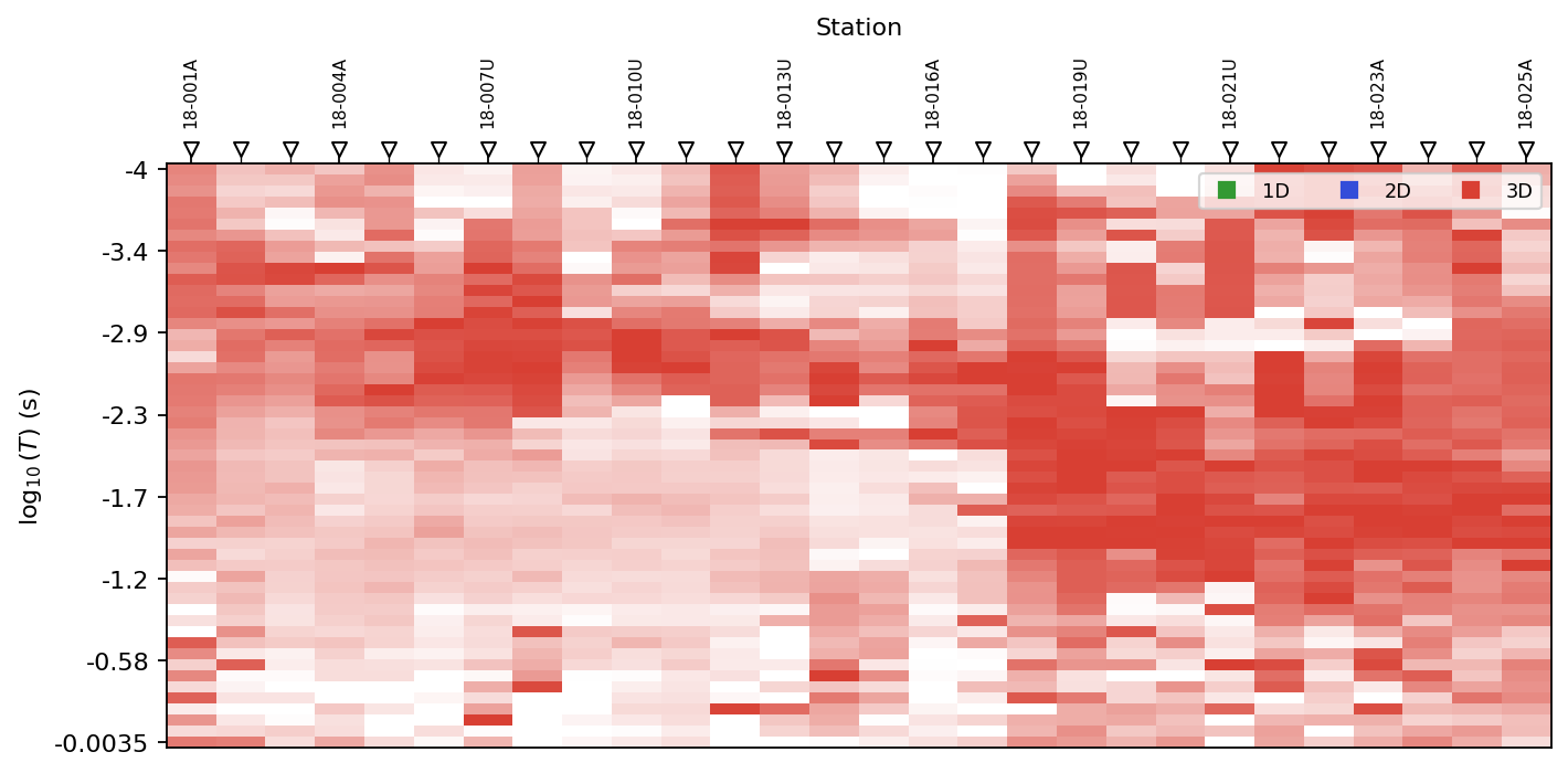
Plot The Dimensionality Grid

plot_dim_confidence_grid maps class labels onto station x period space. Color shows class. Opacity shows a confidence margin from the threshold rule.

import matplotlib.pyplot as plt

from pycsamt.emtools.dimensionality import plot_dim_confidence_grid

fig, ax = plt.subplots(figsize=(9, 4.5))
plot_dim_confidence_grid(
    "data/AMT/WILLY_DATA/L18PLT",
    skew_th=3.0,
    ellipt_th=0.2,
    ax=ax,
)
fig.tight_layout()

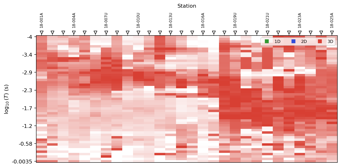
This plot is best for pattern recognition. Look for coherent regions by station and period, not isolated cells.

Plot Period-Band Occupancy

plot_dim_occupancy_area collapses station detail into period-band fractions.

import matplotlib.pyplot as plt

from pycsamt.emtools.dimensionality import plot_dim_occupancy_area

fig, ax = plt.subplots(figsize=(9, 3.8))
plot_dim_occupancy_area(
    "data/AMT/WILLY_DATA/L18PLT",
    skew_th=3.0,
    ellipt_th=0.2,
    n_bands=24,
    ax=ax,
)
fig.tight_layout()

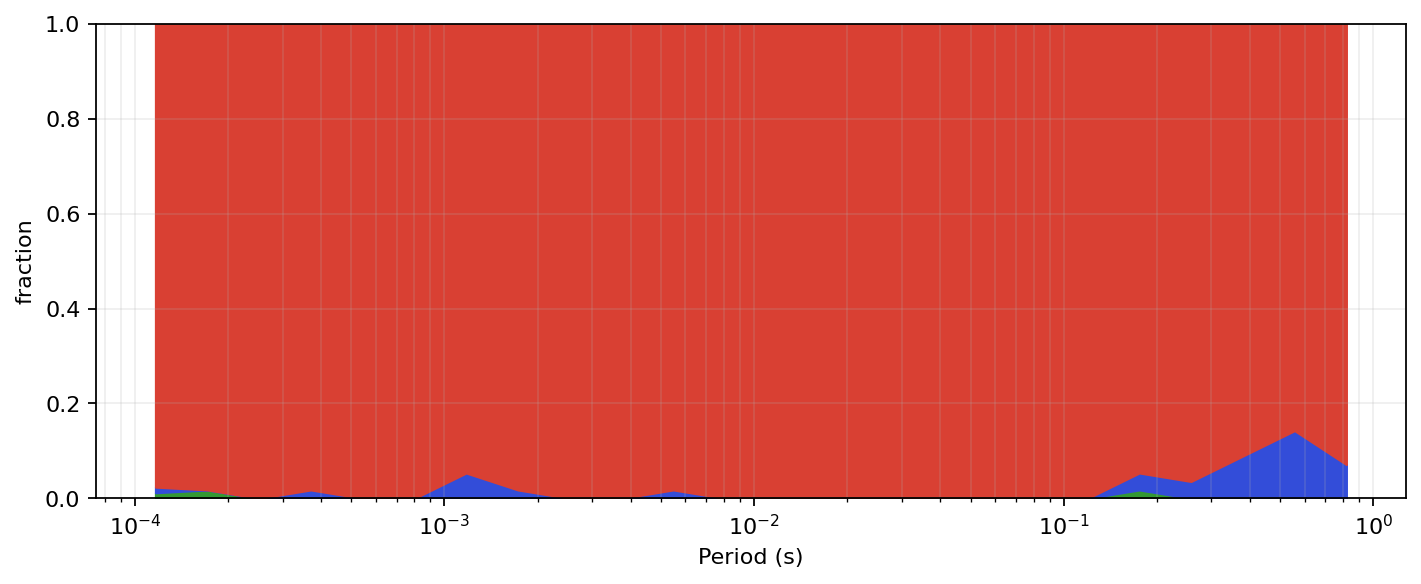
Use this when you need to say whether 3-D behavior is concentrated at short periods, long periods, or spread across the whole band.

Map Dimensionality At One Period

plot_dim_map chooses the nearest available period for each station and maps the dimensionality class in station coordinates.

import matplotlib.pyplot as plt

from pycsamt.emtools.dimensionality import plot_dim_map

fig, ax = plt.subplots(figsize=(8, 6))
plot_dim_map(
    "data/AMT/WILLY_DATA/L18PLT",
    period=0.01,
    skew_th=3.0,
    ellipt_th=0.2,
    ax=ax,
)
fig.tight_layout()

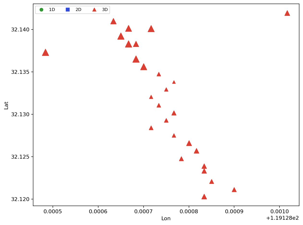
Use this for spatial checks. A line-wide class change is different from one station acting anomalously.

Pre-2D Inversion Assessment

pre2d_inversion_assessment is the audit table to save before a 2-D inversion. It combines dimensionality fractions, strike estimates, strike stability, rotation status, and Groom-Bailey status.

from pycsamt.emtools.dimensionality import pre2d_inversion_assessment

assessment = pre2d_inversion_assessment(
    "data/AMT/WILLY_DATA/L18PLT",
    band=(0.001, 1.0),
    skew_th=3.0,
    ellipt_th=0.2,
    rotation_applied=False,
    rotation_method="consensus",
    groom_bailey_attempted=False,
    groom_bailey_applied=False,
    groom_bailey_reason="Not attempted in this screening run.",
)

print(
    assessment[
        [
            "station",
            "frac_1d",
            "frac_2d",
            "frac_3d",
            "strike_consensus_deg",
            "strike_consensus_iqr_deg",
            "strike_curve_iqr_deg",
            "recommendation",
        ]
    ].head()
)

   station  frac_1d  ...  strike_curve_iqr_deg               recommendation
0  18-001A      0.0  ...                  66.9  review_3d_effects_before_2d
1  18-002U      0.0  ...                  96.0  review_3d_effects_before_2d
2  18-003A      0.0  ...                  65.0  review_3d_effects_before_2d
3  18-004A      0.0  ...                  89.5  review_3d_effects_before_2d
4  18-005U      0.0  ...                  72.1  review_3d_effects_before_2d

[5 rows x 8 columns]

Important columns include:

• period_min_s and period_max_s: assessed period band.

• frac_1d, frac_2d, frac_3d: dimensionality fractions.

• beta_abs_median and beta_abs_p95: skew summary.

• ellipt_abs_median: ellipticity summary.

• strike_sweep_deg: impedance-sweep strike estimate.

• strike_pt_deg: phase-tensor strike estimate.

• strike_consensus_deg and strike_consensus_iqr_deg: combined strike and uncertainty.

• strike_curve_iqr_deg: frequency-dependent strike stability.

• rotated_to_strike and rotation_angle_deg: rotation audit.

• groom_bailey_attempted and groom_bailey_applied: distortion correction audit.

• recommendation: simple screening recommendation.

This table is useful in manuscripts and reports because it records not only the selected strike, but also whether the assumptions behind a 2-D workflow were checked.

Masking 3-D Samples

mask_by_dimensionality replaces samples outside the selected classes with NaN in the impedance tensor and tipper when present.

from pycsamt.emtools.dimensionality import mask_by_dimensionality

masked = mask_by_dimensionality(
    "data/AMT/WILLY_DATA/L18PLT",
    keep=(0, 1),
    inplace=False,
)

By default, keep=(0, 1) keeps 1-D and 2-D samples and masks 3-D samples. Use this carefully: masking can remove large parts of a real survey if the line is strongly 3-D.

Projecting To A 2-D Tensor Form

project_to_2d rotates data to strike and optionally antisymmetrizes the off-diagonal tensor terms.

from pycsamt.emtools.dimensionality import project_to_2d

projected = project_to_2d(
    "data/AMT/WILLY_DATA/L18PLT",
    strike=None,
    method="swift",
    antisym=True,
    inplace=False,
)

When strike=None, pyCSAMT estimates strike before rotation. Pass an explicit strike angle when you have already selected one from your assessment table or a separate structural analysis.

Sparse Dictionary Workflow

The dictionary route learns patterns from four standardized features:

beta_abs
ellipt_abs
logrho_det
tip_amp

It is unsupervised. It does not know geology. It learns atoms that represent repeated feature patterns, encodes each sample with sparse coefficients, and assigns a dimensionality class from the dominant atom.

from pycsamt.emtools.dimensionality import (
    encode_dimensionality,
    learn_dim_dictionary,
)

model = learn_dim_dictionary(
    "data/AMT/WILLY_DATA/L18PLT",
    n_atoms=6,
    lam=0.05,
    n_iter=40,
    code_iter=50,
)

encoded = encode_dimensionality(
    "data/AMT/WILLY_DATA/L18PLT",
    model,
    lam=0.05,
    code_iter=50,
)

print(encoded.filter(regex="station|period|dim_pred|^a").head())

   station    period   a0        a1        a2   a3        a4       a5  dim_pred
0  18-001A  0.000096  0.0 -1.327892  0.896831  0.0  0.016784 -0.00000         1
1  18-001A  0.000115  0.0 -1.317513  0.798761  0.0  0.000000 -0.00000         1
2  18-001A  0.000137  0.0 -1.361449  0.662154  0.0  0.000000 -0.02091         1
3  18-001A  0.000164 -0.0 -1.086200  0.800304 -0.0  0.350492  0.00000         1
4  18-001A  0.000196 -0.0 -0.336239  0.791009 -0.0  0.194019  0.00000         2

The model dictionary contains:

• D: learned atom matrix.

• A: sparse code matrix for the training samples.

• mu and sd: feature standardization values.

• feat: feature names.

• meta: sample metadata such as station names and periods.

The encoded table keeps the feature columns and adds:

• a0, a1, …: sparse atom coefficients.

• dim_pred: dictionary-derived dimensionality label.

Compare Rule Labels And Dictionary Labels

The dictionary workflow is most useful as an independent check, not as a replacement for the rule.

import pandas as pd

from pycsamt.emtools.dimensionality import (
    classify_dimensionality,
    encode_dimensionality,
    learn_dim_dictionary,
)

survey = "data/AMT/WILLY_DATA/L18PLT"
rule = classify_dimensionality(survey)
model = learn_dim_dictionary(survey, n_atoms=6)
encoded = encode_dimensionality(survey, model)

compare = rule[["station", "period", "dim"]].merge(
    encoded[["station", "period", "dim_pred"]],
    on=["station", "period"],
    how="inner",
)
agreement = (compare["dim"] == compare["dim_pred"]).mean()
print(f"rule/dictionary agreement = {agreement:.2%}")

rule/dictionary agreement = 68.13%

Agreement near 100 percent means the learned atoms reproduce the rule. Lower agreement means the data-driven features are separating samples differently. That can be useful, but it needs interpretation.

Dictionary Masking And Atom Plots

mask_by_dictionary applies the same idea as mask_by_dimensionality but uses dim_pred from the learned dictionary. plot_atom_psection shows which learned atom dominates each station-period cell.

import matplotlib.pyplot as plt

from pycsamt.emtools.dimensionality import (
    learn_dim_dictionary,
    mask_by_dictionary,
    plot_atom_psection,
)

survey = "data/AMT/WILLY_DATA/L18PLT"
model = learn_dim_dictionary(survey, n_atoms=6)

masked = mask_by_dictionary(
    survey,
    model,
    keep=(0, 1),
    inplace=False,
)

fig, ax = plt.subplots(figsize=(9, 4.8))
plot_atom_psection(survey, model, energy="l2", ax=ax)
fig.tight_layout()

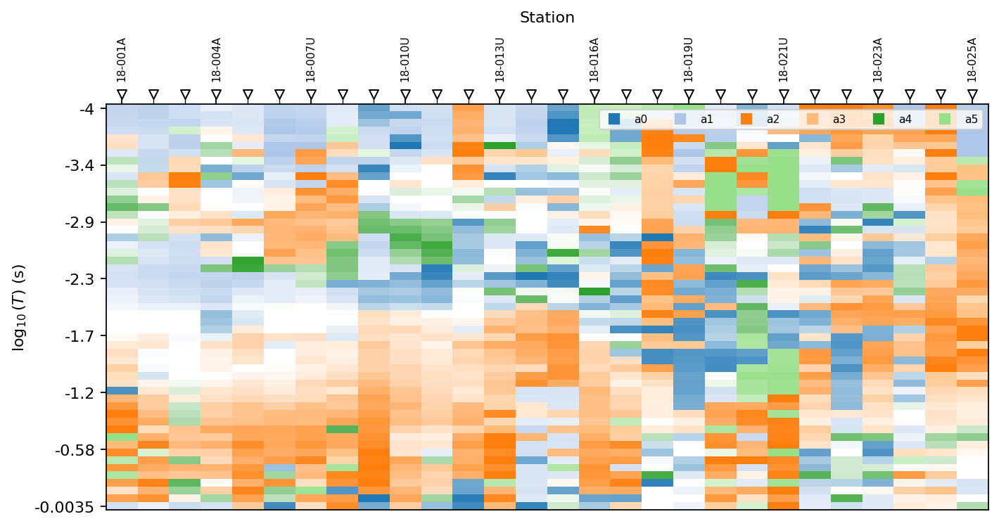
Use the atom pseudo-section to check whether one learned pattern is localized in a period band or station group. A model that produces random-looking atom occupancy is not a useful diagnostic.

Reading The Results

Use this interpretation order:

• Inspect beta_abs and ellipt_abs before accepting labels.

• Report the thresholds used for rule-based classification.

• Sweep thresholds when the conclusion depends on the default values.

• Treat broad station-period patterns as stronger evidence than isolated cells.

• Save pre2d_inversion_assessment before a 2-D inversion.

• Use dictionary labels as an independent check, not as a black-box replacement for the phase-tensor rule.

Common Failure Modes

Mostly 3-D classifications

This may be a real survey property, especially in complex geology. Do a threshold sweep before changing thresholds to get the result you hoped for.

No tipper data

tip_amp becomes NaN. The dictionary workflow replaces missing values during standardization, but you should still record that tipper information was absent.

Unstable strike

A wide strike_consensus_iqr_deg or strike_curve_iqr_deg means strike is not stable across methods or period. Review the band before rotating to 2-D.

Masking removes too much data

If most samples are 3-D, keep=(0, 1) may leave too little for a stable inversion. Consider changing the period band rather than masking blindly.

Dictionary disagreement

Rule and dictionary labels can disagree because they use different information. Inspect atom occupancy and feature distributions before using dictionary masks operationally.

Saving A Reproducible Bundle

For reporting, save the raw features, rule labels, pre-2D assessment, and dictionary encoding.

from pathlib import Path

import matplotlib.pyplot as plt

from pycsamt.emtools.dimensionality import (
    classify_dimensionality,
    encode_dimensionality,
    learn_dim_dictionary,
    phase_features_table,
    plot_dim_confidence_grid,
    pre2d_inversion_assessment,
)

survey = "data/AMT/WILLY_DATA/L18PLT"
out = Path("outputs/dimensionality_l18plt")
out.mkdir(parents=True, exist_ok=True)

features = phase_features_table(survey)
rule = classify_dimensionality(survey)
assessment = pre2d_inversion_assessment(survey, band=(0.001, 1.0))
model = learn_dim_dictionary(survey, n_atoms=6)
encoded = encode_dimensionality(survey, model)

features.to_csv(out / "phase_features.csv", index=False)
rule.to_csv(out / "rule_dimensionality.csv", index=False)
assessment.to_csv(out / "pre2d_assessment.csv", index=False)
encoded.to_csv(out / "dictionary_encoding.csv", index=False)

fig, ax = plt.subplots(figsize=(9, 4.5))
plot_dim_confidence_grid(survey, ax=ax)
fig.tight_layout()
fig.savefig(out / "dimensionality_confidence_grid.png", dpi=200)

Worked Example

The gallery example uses L18PLT from data/AMT/WILLY_DATA/. It starts from one-station skew and ellipticity curves, shows the rule-based feature-space partition, sweeps thresholds, plots the pseudo-section and occupancy views, checks 2-D projection, and compares rule-based labels with dictionary-learned labels.

Open the rendered example here: Phase-tensor dimensionality: rule-based and dictionary-learned (pycsamt.emtools.dimensionality).